5. Nonlinear System Modeling, Analysis, and Design

The Python Control Systems Library contains a variety of tools for modeling, analyzing, and designing nonlinear feedback systems, including support for simulation and optimization. This chapter describes the primary functionality available, both in the core python-control package and in specialized modules and subpackages.

5.1. Nonlinear System Models

Nonlinear input/output systems are represented as state space systems of the form

$\frac{dx}{dt} &= f(t, x, u, \theta), \\ y &= h(t, x, u, \theta),$

where $t$ represents the current time, $x \in \mathbb{R}^n$ is the system state, $u \in \mathbb{R}^m$ is the system input, $y \in \mathbb{R}^p$ is the system output, and $\theta$ represents a set of parameters.

Discrete time systems are also supported and have dynamics of the form

$x[t+1] &= f(t, x[t], u[t], \theta), \\ y[t] &= h(t, x[t], u[t], \theta).$

A nonlinear input/output model is said to be “static” if the output $y(t)$ at any given time $t$ depends only on the input $u(t)$ at that same time $t$ and not on past or future values of $u$ .

Creating nonlinear models

A nonlinear system is created using the nlsys() factory function:

sys = ct.nlsys(
    updfcn[, outfcn], inputs=m, states=n, outputs=p, [, params=params])

The updfcn argument is a function returning the state update function:

updfcn(t, x, u, params) -> array

where t is a float representing the current time, x is a 1-D array with shape (n,), u is a 1-D array with shape (m,), and params is a dict containing the values of parameters used by the function. The dynamics of the system can be in continuous or discrete time (use the dt keyword to create a discrete-time system).

The output function outfcn is used to specify the outputs of the system and has the same calling signature as updfcn. If it is not specified, then the output of the system is set equal to the system state. Otherwise, it should return an array of shape (p,). If a input/output system is static, the state x should still be passed to the output function, but the state is ignored.

Note that the number of states, inputs, and outputs should generally be explicitly specified, although some operations can infer the dimensions if they are not given when the system is created. The inputs, outputs, and states keywords can also be given as lists of strings, in which case the various signals will be given the appropriate names.

To illustrate the creation of a nonlinear I/O system model, consider a simple model of a spring loaded arm driven by a motor:

The dynamics of this system can be modeled using the following code:

# Parameter values
servomech_params = {
    'J': 100,             # Moment of inertia of the motor
    'b': 10,              # Angular damping of the arm
    'k': 1,               # Spring constant
    'r': 1,               # Location of spring contact on arm
    'l': 2,               # Distance to the read head
}

# State derivative
def servomech_update(t, x, u, params):
    # Extract the configuration and velocity variables from the state vector
    theta = x[0]                # Angular position of the disk drive arm
    thetadot = x[1]             # Angular velocity of the disk drive arm
    tau = u[0]                  # Torque applied at the base of the arm

    # Get the parameter values
    J, b, k, r = map(params.get, ['J', 'b', 'k', 'r'])

    # Compute the angular acceleration
    dthetadot = 1/J * (
        -b * thetadot - k * r * np.sin(theta) + tau)

    # Return the state update law
    return np.array([thetadot, dthetadot])

# System output (tip radial position + angular velocity)
def servomech_output(t, x, u, params):
    l = params['l']
    return np.array([l * x[0], x[1]])

# System dynamics
servomech = ct.nlsys(
    servomech_update, servomech_output, name='servomech',
    params=servomech_params, states=['theta', 'thdot'],
    outputs=['y', 'thdot'], inputs=['tau'])

A summary of the model can be obtained using the string representation of the model (via the Python print function):

>>> print(servomech)
<NonlinearIOSystem>: servomech
Inputs (1): ['tau']
Outputs (2): ['y', 'thdot']
States (2): ['theta', 'thdot']
Parameters: ['J', 'b', 'k', 'r', 'l']

Update: <function servomech_update at ...>
Output: <function servomech_output at ...>

Operating points and linearization

A nonlinear input/output system can be linearized around an equilibrium point to obtain a StateSpace linear system:

sys_ss = ct.linearize(sys_nl, xeq, ueq)

If the equilibrium point is not known, the find_operating_point() function can be used to obtain an equilibrium point. In its simplest form, find_operating_point finds an equilibrium point given either the desired input or desired output:

xeq, ueq = find_operating_point(sys, x0, u0)
xeq, ueq = find_operating_point(sys, x0, u0, y0)

The first form finds an equilibrium point for a given input u0 based on an initial guess x0. The second form fixes the desired output values y0 and uses x0 and u0 as an initial guess to find the equilibrium point. If no equilibrium point can be found, the function returns the operating point that minimizes the state update (state derivative for continuous-time systems, state difference for discrete time systems).

More complex operating points can be found by specifying which states, inputs, or outputs should be used in computing the operating point, as well as desired values of the states, inputs, outputs, or state updates. See the find_operating_point() documentation for more details.

Simulations and plotting

To simulate an input/output system, use the input_output_response() function:

resp = ct.input_output_response(sys_nl, timepts, U, x0, params)
t, y, x = resp.time, resp.outputs, resp.states

Time responses can be plotted using the time_response_plot() function or (equivalently) the TimeResponseData.plot() method:

cplt = ct.time_response_plot(resp)  # function call
cplt = resp.plot()                  # method call

The resulting ControlPlot object can be used to access different plot elements:

cplt.lines: Array of matplotlib.lines.Line2D objects for each line in the plot. The shape of the array matches the subplots shape and the value of the array is a list of Line2D objects in that subplot.
cplt.axes: 2D array of matplotlib.axes.Axes for the plot.
cplt.figure: matplotlib.figure.Figure containing the plot.
cplt.legend: legend object(s) contained in the plot.

The combine_time_responses() function an be used to combine multiple time responses into a single TimeResponseData object:

timepts = np.linspace(0, 10)

U1 = np.sin(timepts)
resp1 = ct.input_output_response(servomech, timepts, U1)

U2 = np.cos(2*timepts)
resp2 = ct.input_output_response(servomech, timepts, U2)

resp = ct.combine_time_responses(
    [resp1, resp2], trace_labels=["Scenario #1", "Scenario #2"])
resp.plot(legend_loc=False)

Nonlinear system properties

The following basic attributes and methods are available for NonlinearIOSystem objects:

`dynamics`(t, x, u[, params])	Dynamics of a differential or difference equation.
`output`(t, x, u[, params])	Compute the output of the system.
`linearize`(x0[, u0, t, params, eps, copy_names])	Linearize an input/output system at a given state and input.
`__call__`(u[, params, squeeze])	Evaluate a (static) nonlinearity at a given input value.

The dynamics() method returns the right hand side of the differential or difference equation, evaluated at the current time, state, input, and (optionally) parameter values. The output() method returns the system output. For static nonlinear systems, it is also possible to obtain the value of the output by directly calling the system with the value of the input:

>>> sys = ct.nlsys(
...    None, lambda t, x, u, params: np.sin(u), inputs=1, outputs=1)
>>> sys(1)
np.float64(0.8414709848078965)

The NonlinearIOSystem.linearize() method is equivalent to the linearize() function.

5.2. Phase Plane Plots

Insight into nonlinear systems can often be obtained by looking at phase plane diagrams. The phase_plane_plot() function allows the creation of a 2-dimensional phase plane diagram for a system. This functionality is supported by a set of mapping functions that are part of the phaseplot module.

The default method for generating a phase plane plot is to provide a 2D dynamical system along with a range of coordinates in phase space:

def sys_update(t, x, u, params):
    return np.array([[0, 1], [-1, -1]]) @ x
sys = ct.nlsys(
    sys_update, states=['position', 'velocity'],
    inputs=0, name='damped oscillator')
axis_limits = [-1, 1, -1, 1]
ct.phase_plane_plot(sys, axis_limits)

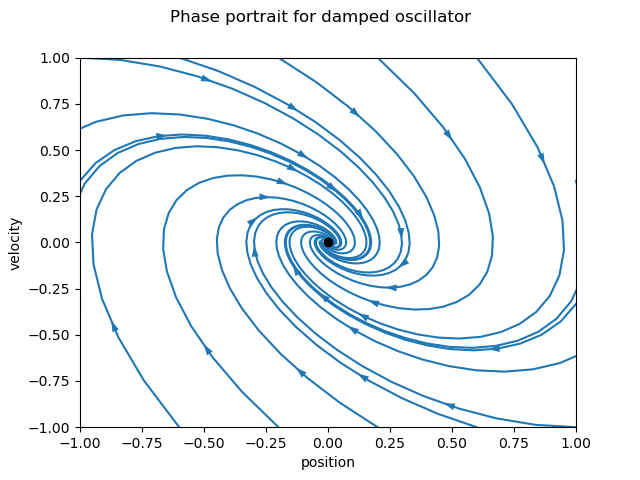
By default the plot includes streamlines infered from function values on a grid, equilibrium points and separatrices if they exist. A variety of options are available to modify the information that is plotted, including plotting a grid of vectors instead of streamlines, plotting streamlines from arbitrary starting points and turning on and off various features of the plot.

To illustrate some of these possibilities, consider a phase plane plot for an inverted pendulum system, which is created using a mesh grid:

def invpend_update(t, x, u, params):
    m, l, b, g = params['m'], params['l'], params['b'], params['g']
    return [x[1], -b/m * x[1] + (g * l / m) * np.sin(x[0]) + u[0]/m]
invpend = ct.nlsys(invpend_update, states=2, inputs=1, name='invpend')

ct.phase_plane_plot(
    invpend, [-2 * np.pi, 2 * np.pi, -2, 2],
    params={'m': 1, 'l': 1, 'b': 0.2, 'g': 1})
plt.xlabel(r"$\theta$ [rad]")
plt.ylabel(r"$\dot\theta$ [rad/sec]")

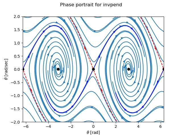
This figure shows several features of more complex phase plane plots: multiple equilibrium points are shown, with saddle points showing separatrices, and streamlines generated generated from a rectangular 25x25 grid (default) of function evaluations. Together, the multiple features in the phase plane plot give a good global picture of the topological structure of solutions of the dynamical system.

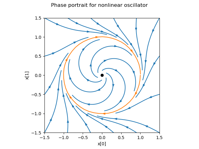
Phase plots can be built up by hand using a variety of helper functions that are part of the phaseplot (pp) module. For more precise control, the streamlines can also generated by integrating the system forwards or backwards in time from a set of initial conditions. The initial conditions can be chosen on a rectangular grid, rectangual boundary, circle or from an arbitrary set of points.

import control.phaseplot as pp

def oscillator_update(t, x, u, params):
    return [x[1] + x[0] * (1 - x[0]**2 - x[1]**2),
            -x[0] + x[1] * (1 - x[0]**2 - x[1]**2)]
oscillator = ct.nlsys(
    oscillator_update, states=2, inputs=0, name='nonlinear oscillator')

ct.phase_plane_plot(oscillator, [-1.5, 1.5, -1.5, 1.5], 0.9,
    plot_streamlines=True)
pp.streamlines(
    oscillator, np.array([[0, 0]]), 1.5,
    gridtype='circlegrid', gridspec=[0.5, 6], dir='both')
pp.streamlines(
    oscillator, np.array([[1, 0]]), 2 * np.pi, arrows=6, color='b')
plt.gca().set_aspect('equal')

_images/phaseplot-oscillator-helpers.png

The following helper functions are available:

`phaseplot.equilpoints`(sys, pointdata[, ...])	Plot equilibrium points in the phase plane.
`phaseplot.separatrices`(sys, pointdata[, ...])	Plot separatrices in the phase plane.
`phaseplot.streamlines`(sys, pointdata[, ...])	Plot stream lines in the phase plane.
`phaseplot.streamplot`(sys, pointdata[, ...])	Plot streamlines in the phase plane.
`phaseplot.vectorfield`(sys, pointdata[, ...])	Plot a vector field in the phase plane.

The phase_plane_plot() function calls these helper functions based on the options it is passed.

Note that unlike other plotting functions, phase plane plots do not involve computing a response and then plotting the result via a plot() method. Instead, the plot is generated directly be a call to the phase_plane_plot() function (or one of the phaseplot helper functions).

5.3. Optimization-Based Control

The optimal module contains a set of classes and functions that can be used to solve optimal control and optimal estimation problems for linear or nonlinear systems. The objects in this module must be explicitly imported:

import control as ct
import control.optimal as opt

Optimal control problem setup

Consider the optimal control problem:

$\min_{u(\cdot)} \int_0^T L(x,u)\, dt + V \bigl( x(T) \bigr)$

subject to the constraint

$\dot x = f(x, u), \qquad x\in\mathbb{R}^n,\, u\in\mathbb{R}^m.$

Abstractly, this is a constrained optimization problem where we seek a feasible trajectory $(x(t), u(t))$ that minimizes the cost function

$J(x, u) = \int_0^T L(x, u)\, dt + V \bigl( x(T) \bigr).$

More formally, this problem is equivalent to the “standard” problem of minimizing a cost function $J(x, u)$ where $(x, u) \in L_2[0,T]$ (the set of square integrable functions) and $h(z) = \dot x(t) - f(x(t), u(t)) = 0$ models the dynamics. The term $L(x, u)$ is referred to as the integral (or trajectory) cost and $V(x(T))$ is the final (or terminal) cost.

It is often convenient to ask that the final value of the trajectory, denoted $x_\text{f}$ , be specified. We can do this by requiring that $x(T) = x_\text{f}$ or by using a more general form of constraint:

$\psi_i(x(T)) = 0, \qquad i = 1, \dots, q.$

The fully constrained case is obtained by setting $q = n$ and defining $\psi_i(x(T)) = x_i(T) - x_{i,\text{f}}$ . For a control problem with a full set of terminal constraints, $V(x(T))$ can be omitted (since its value is fixed).

Finally, we may wish to consider optimizations in which either the state or the inputs are constrained by a set of nonlinear functions of the form

$\text{lb}_i \leq g_i(x, u) \leq \text{ub}_i, \qquad i = 1, \dots, k.$

where $\text{lb}_i$ and $\text{ub}_i$ represent lower and upper bounds on the constraint function $g_i$ . Note that these constraints can be on the input, the state, or combinations of input and state, depending on the form of $g_i$ . Furthermore, these constraints are intended to hold at all instants in time along the trajectory.

For a discrete-time system, the same basic formulation applies except that the cost function is given by

$J(x, u) = \sum_{k=0}^{N-1} L(x_k, u_k)\, dt + V(x_N).$

A common use of optimization-based control techniques is the implementation of model predictive control (MPC, also called receding horizon control). In model predictive control, a finite horizon optimal control problem is solved, generating open-loop state and control trajectories. The resulting control trajectory is applied to the system for a fraction of the horizon length. This process is then repeated, resulting in a sampled data feedback law. This approach is illustrated in the following figure:

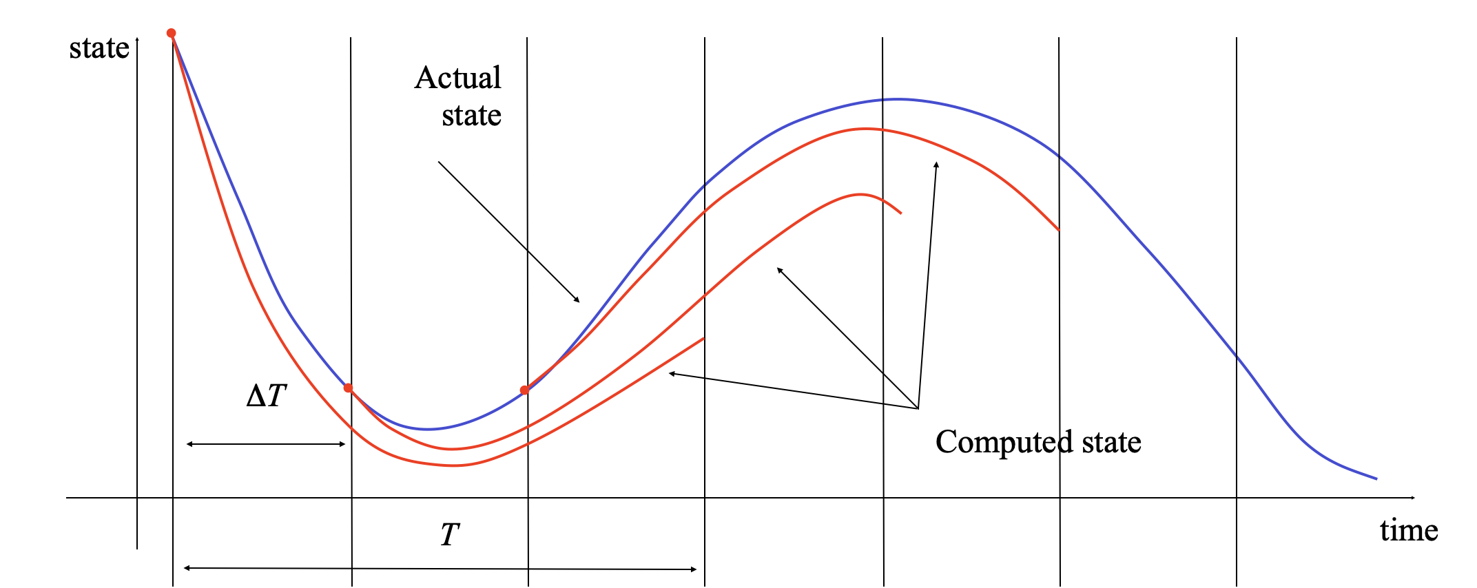
Every $\Delta T$ seconds, an optimal control problem is solved over a $T$ second horizon, starting from the current state. The first $\Delta T$ seconds of the optimal control $u_T^{\*}(\cdot; x(t))$ is then applied to the system. If we let $x_T^{\*}(\cdot; x(t))$ represent the optimal trajectory starting from $x(t)$ then the system state evolves from $x(t)$ at current time $t$ to $x_T^{*}(\Delta T, x(t))$ at the next sample time $t + \Delta T$ , assuming no model uncertainty.

In reality, the system will not follow the predicted path exactly, so that the red (computed) and blue (actual) trajectories will diverge. We thus recompute the optimal path from the new state at time $t + \Delta T$ , extending our horizon by an additional $\Delta T$ units of time. This approach can be shown to generate stabilizing control laws under suitable conditions (see, for example, the FBS2e supplement on Optimization-Based Control).

Module usage

The optimization-based control module provides a means of computing optimal trajectories for nonlinear systems and implementing optimization-based controllers, including model predictive control. It follows the basic problem setups described above, but carries out all computations in discrete time (so that integrals become sums) and over a finite horizon. To access the optimal control modules, import control.optimal:

import control.optimal as opt

To describe an optimal control problem we need an input/output system, a time horizon, a cost function, and (optionally) a set of constraints on the state and/or input, along the trajectory and/or at the terminal time. The optimal control module operates by converting the optimal control problem into a standard optimization problem that can be solved by scipy.optimize.minimize(). The optimal control problem can be solved by using the solve_optimal_trajectory() function:

res = opt.solve_optimal_trajectory(sys, timepts, X0, cost, constraints)

The sys parameter should be an InputOutputSystem and the timepts parameter should represent a time vector that gives the list of times at which the cost and constraints should be evaluated (the time points need not be uniformly spaced).

The cost function has call signature cost(t, x, u) and should return the (incremental) cost at the given time, state, and input. It will be evaluated at each point in the timepts vector. The terminal_cost parameter can be used to specify a cost function for the final point in the trajectory.

The constraints parameter is a list of constraints similar to that used by the scipy.optimize.minimize() function. Each constraint is specified using one of the following forms:

LinearConstraint(A, lb, ub)
NonlinearConstraint(f, lb, ub)

For a linear constraint, the 2D array A is multiplied by a vector consisting of the current state x and current input u stacked vertically, then compared with the upper and lower bound. This constraint is satisfied if

lb <= A @ np.hstack([x, u]) <= ub

A nonlinear constraint is satisfied if

lb <= f(x, u) <= ub

The constraints are taken as trajectory constraints holding at all points on the trajectory. The terminal_constraints parameter can be used to specify a constraint that only holds at the final point of the trajectory.

The return value for solve_optimal_trajectory() is a bundle object that has the following elements:

res.success: True if the optimization was successfully solved

res.inputs: optimal input

res.states: state trajectory (if return_x was True)

res.time: copy of the time timepts vector

In addition, the results from scipy.optimize.minimize() are also available as additional attributes, as described in scipy.optimize.OptimizeResult.

To simplify the specification of cost functions and constraints, the optimal module defines a number of utility functions for optimal control problems:

`optimal.quadratic_cost`(sys, Q, R[, x0, u0])	Create quadratic cost function.
`optimal.input_poly_constraint`(sys, A, b)	Create input constraint from polytope.
`optimal.input_range_constraint`(sys, lb, ub)	Create input constraint from polytope.
`optimal.output_poly_constraint`(sys, A, b)	Create output constraint from polytope.
`optimal.output_range_constraint`(sys, lb, ub)	Create output constraint from range.
`optimal.state_poly_constraint`(sys, A, b)	Create state constraint from polytope.
`optimal.state_range_constraint`(sys, lb, ub)	Create state constraint from range.

Example

Consider the vehicle steering example described in Example 2.3 of Optimization-Based Control (OBC). The dynamics of the system can be defined as a nonlinear input/output system using the following code:

import matplotlib.pyplot as plt
import numpy as np
import control as ct
import control.optimal as opt

def vehicle_update(t, x, u, params):
    # Get the parameters for the model
    l = params.get('wheelbase', 3.)         # vehicle wheelbase
    phimax = params.get('maxsteer', 0.5)    # max steering angle (rad)

    # Saturate the steering input
    phi = np.clip(u[1], -phimax, phimax)

    # Return the derivative of the state
    return np.array([
        np.cos(x[2]) * u[0],            # xdot = cos(theta) v
        np.sin(x[2]) * u[0],            # ydot = sin(theta) v
        (u[0] / l) * np.tan(phi)        # thdot = v/l tan(phi)
    ])

def vehicle_output(t, x, u, params):
    return x                            # return x, y, theta (full state)

# Define the vehicle steering dynamics as an input/output system
vehicle = ct.NonlinearIOSystem(
    vehicle_update, vehicle_output, states=3, name='vehicle',
    inputs=('v', 'phi'), outputs=('x', 'y', 'theta'))

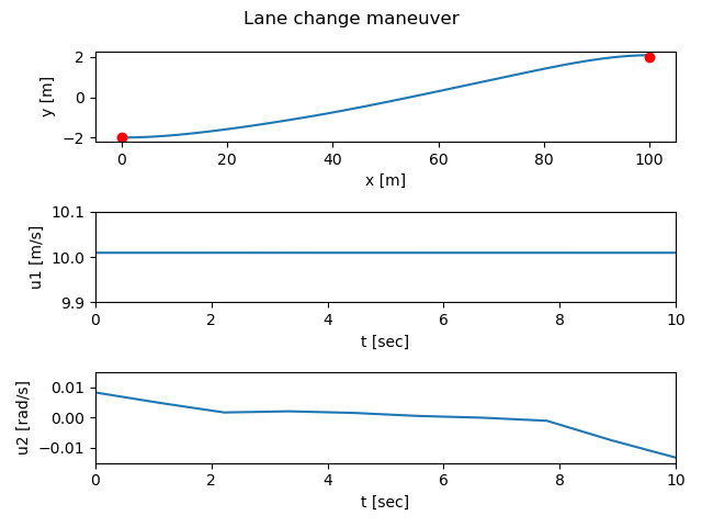
We consider an optimal control problem that consists of “changing lanes” by moving from the point x = 0 m, y = -2 m, $\theta$ = 0 to the point x = 100 m, y = 2 m, $\theta$ = 0) over a period of 10 seconds and with a starting and ending velocity of 10 m/s:

x0 = np.array([0., -2., 0.]); u0 = np.array([10., 0.])
xf = np.array([100., 2., 0.]); uf = np.array([10., 0.])
Tf = 10

To set up the optimal control problem we design a cost function that penalizes the state and input using quadratic cost functions:

Q = np.diag([0, 0, 0.1])          # don't turn too sharply
R = np.diag([1, 1])               # keep inputs small
P = np.diag([1000, 1000, 1000])   # get close to final point
traj_cost = opt.quadratic_cost(vehicle, Q, R, x0=xf, u0=uf)
term_cost = opt.quadratic_cost(vehicle, P, 0, x0=xf)

We also constrain the maximum turning rate to 0.1 radians (about 6 degrees) and constrain the velocity to be in the range of 9 m/s to 11 m/s:

constraints = [ opt.input_range_constraint(vehicle, [8, -0.1], [12, 0.1]) ]

Finally, we solve for the optimal inputs:

timepts = np.linspace(0, Tf, 10, endpoint=True)
result = opt.solve_optimal_trajectory(
    vehicle, timepts, x0, traj_cost, constraints,
    terminal_cost=term_cost, initial_guess=u0)

Plotting the results:

# Simulate the system dynamics (open loop)
resp = ct.input_output_response(
    vehicle, timepts, result.inputs, x0,
    evaluation_times=np.linspace(0, Tf, 100))
t, y, u = resp.time, resp.outputs, resp.inputs

plt.subplot(3, 1, 1)
plt.plot(y[0], y[1])
plt.plot(x0[0], x0[1], 'ro', xf[0], xf[1], 'ro')
plt.xlabel("x [m]")
plt.ylabel("y [m]")

plt.subplot(3, 1, 2)
plt.plot(t, u[0])
plt.axis([0, 10, 9.9, 10.1])
plt.xlabel("t [sec]")
plt.ylabel("u1 [m/s]")

plt.subplot(3, 1, 3)
plt.plot(t, u[1])
plt.axis([0, 10, -0.015, 0.015])
plt.xlabel("t [sec]")
plt.ylabel("u2 [rad/s]")

plt.suptitle("Lane change maneuver")
plt.tight_layout()

yields

Optimization Tips

The python-control optimization module makes use of the SciPy optimization toolbox and it can sometimes be tricky to get the optimization to converge. If you are getting errors when solving optimal control problems or your solutions do not seem close to optimal, here are a few things to try:

The initial guess matters: providing a reasonable initial guess is often needed in order for the optimizer to find a good answer. For an optimal control problem that uses a larger terminal cost to get to a neighborhood of a final point, a straight line in the state space often works well.
Less is more: try using a smaller number of time points in your optimization. The default optimal control problem formulation uses the value of the inputs at each time point as a free variable and this can generate a large number of parameters quickly. Often you can find very good solutions with a small number of free variables (the example above uses 3 time points for 2 inputs, so a total of 6 optimization variables). Note that you can “resample” the optimal trajectory by running a simulation of the system and using the t_eval keyword in input_output_response (as done above).
Use a smooth basis: as an alternative to parameterizing the optimal control inputs using the value of the control at the listed time points, you can specify a set of basis functions using the basis keyword in solve_optimal_trajectory() and then parameterize the controller by linear combination of the basis functions. The flatsys subpackage defines several sets of basis functions that can be used.
Tweak the optimizer: by using the minimize_method, minimize_options, and minimize_kwargs keywords in solve_optimal_trajectory(), you can choose the SciPy optimization function that you use and set many parameters. See scipy.optimize.minimize() for more information on the optimizers that are available and the options and keywords that they accept.
Walk before you run: try setting up a simpler version of the optimization, remove constraints or simplifying the cost to get a simple version of the problem working and then add complexity. Sometimes this can help you find the right set of options or identify situations in which you are being too aggressive in what you are trying to get the system to do.

See Optimal control for vehicle steering (lane change) for some examples of different problem formulations.

Module classes and functions

The following classes and functions are defined in the optimal module:

`optimal.OptimalControlProblem`(sys, timepts, ...)	Description of a finite horizon, optimal control problem.
`optimal.OptimalControlResult`(ocp, res[, ...])	Result from solving an optimal control problem.
`optimal.OptimalEstimationProblem`(sys, ...[, ...])	Description of a finite horizon, optimal estimation problem.
`optimal.OptimalEstimationResult`(oep, res[, ...])	Result from solving an optimal estimation problem.

`optimal.create_mpc_iosystem`(sys, timepts[, ...])	Create a model predictive I/O control system.
`optimal.disturbance_range_constraint`(sys, lb, ub)	Create constraint for bounded disturbances.
`optimal.gaussian_likelihood_cost`(sys, Rv[, Rw])	Create cost function for Gaussian likelihoods.
`optimal.input_poly_constraint`(sys, A, b)	Create input constraint from polytope.
`optimal.input_range_constraint`(sys, lb, ub)	Create input constraint from polytope.
`optimal.output_poly_constraint`(sys, A, b)	Create output constraint from polytope.
`optimal.output_range_constraint`(sys, lb, ub)	Create output constraint from range.
`optimal.quadratic_cost`(sys, Q, R[, x0, u0])	Create quadratic cost function.
`optimal.solve_optimal_trajectory`(sys, timepts)	Compute the solution to an optimal control problem.
`optimal.solve_optimal_estimate`(sys, timepts)	Compute the solution to a finite horizon estimation problem.
`optimal.state_poly_constraint`(sys, A, b)	Create state constraint from polytope.
`optimal.state_range_constraint`(sys, lb, ub)	Create state constraint from range.

5.4. Describing Functions

For nonlinear systems consisting of a feedback connection between a linear system and a nonlinearity, it is possible to obtain a generalization of Nyquist’s stability criterion based on the idea of describing functions. The basic concept involves approximating the response of a nonlinearity to an input $u = A e^{j \omega t}$ as an output $y = N(A) (A e^{j \omega t})$ , where $N(A) \in \mathbb{C}$ represents the (amplitude-dependent) gain and phase associated with the nonlinearity.

In the most common case, the nonlinearity will be a static, time-invariant nonlinear function $y = h(u)$ . However, describing functions can be defined for nonlinear input/output systems that have some internal memory, such as hysteresis or backlash. For simplicity, we take the nonlinearity to be static (memoryless) in the description below, unless otherwise specified.

Stability analysis of a linear system $H(s)$ with a feedback nonlinearity $F(x)$ is done by looking for amplitudes $A$ and frequencies $\omega$ such that

$H(j\omega) N(A) = -1$

If such an intersection exists, it indicates that there may be a limit cycle of amplitude $A$ with frequency $\omega$ .

Describing function analysis is a simple method, but it is approximate because it assumes that higher harmonics can be neglected. More information on describing functions can be found in Feedback Systems, Section 10.5 (Generalized Notions of Gain and Phase).

Module usage

The function describing_function() can be used to compute the describing function of a nonlinear function:

N = ct.describing_function(F, A)

where F is a scalar nonlinear function.

Stability analysis using describing functions is done by looking for amplitudes $A$ and frequencies $\omega$ such that

$H(j\omega) = \frac{-1}{N(A)}$

These points can be determined by generating a Nyquist plot in which the transfer function $H(j\omega)$ intersects the negative reciprocal of the describing function $N(A)$ . The describing_function_response() function computes the amplitude and frequency of any points of intersection:

dfresp = ct.describing_function_response(H, F, amp_range[, omega_range])
dfresp.intersections        # frequency, amplitude pairs

A Nyquist plot showing the describing function and the intersections with the Nyquist curve can be generated using dfresp.plot(), which calls the describing_function_plot() function.

Pre-defined nonlinearities

To facilitate the use of common describing functions, the following nonlinearity constructors are predefined:

friction_backlash_nonlinearity(b)     # backlash nonlinearity with width b
relay_hysteresis_nonlinearity(b, c)   # relay output of amplitude b with
                                      # hysteresis of half-width c
saturation_nonlinearity(ub[, lb])     # saturation nonlinearity with upper
                                      # bound and (optional) lower bound

Calling these functions will create an object F that can be used for describing function analysis. For example, to create a saturation nonlinearity:

F = ct.saturation_nonlinearity(1)

These functions use the DescribingFunctionNonlinearity class, which allows an analytical description of the describing function.

Example

The following example demonstrates a more complicated interaction between a (non-static) nonlinearity and a higher order transfer function, resulting in multiple intersection points:

# Linear dynamics
H_simple = ct.tf([1], [1, 2, 2, 1])
H_multiple = ct.tf(H_simple * ct.tf(*ct.pade(5, 4)) * 4, name='sys')
omega = np.logspace(-3, 3, 500)

# Nonlinearity
F_backlash = ct.friction_backlash_nonlinearity(1)
amp = np.linspace(0.6, 5, 50)

# Describing function plot
cplt = ct.describing_function_plot(
    H_multiple, F_backlash, amp, omega, mirror_style=False)

Module classes and functions

`describing_function`(F, A[, num_points, ...])	Numerically compute describing function of a nonlinear function.
`describing_function_response`(H, F, A[, ...])	Compute the describing function response of a system.
`describing_function_plot`(data, args, *kwargs)	Nyquist plot with describing function for a nonlinear system.
`DescribingFunctionNonlinearity`()	Base class for nonlinear systems with a describing function.
`friction_backlash_nonlinearity`(b)	Backlash nonlinearity for describing function analysis.
`relay_hysteresis_nonlinearity`(b, c)	Relay w/ hysteresis for describing function analysis.
`saturation_nonlinearity`([ub, lb])	Saturation nonlinearity for describing function analysis.
`__call__`(A)	Evaluate the nonlinearity at a (scalar) input value.

5.5. Differentially Flat Systems

The flatsys subpackage contains a set of classes and functions to compute trajectories for differentially flat systems. The objects in this subpackage must be explicitly imported:

import control as ct
import control.flatsys as fs

Overview of differential flatness

A nonlinear differential equation of the form

$\dot x = f(x, u), \qquad x \in R^n, u \in R^m$

is differentially flat if there exists a function $\alpha$ such that

$z = \alpha(x, u, \dot u\, \dots, u^{(p)})$

and we can write the solutions of the nonlinear system as functions of $z$ and a finite number of derivatives

(1) $x &= \beta(z, \dot z, \dots, z^{(q)}) \\ u &= \gamma(z, \dot z, \dots, z^{(q)}).$

For a differentially flat system, all of the feasible trajectories for the system can be written as functions of a flat output $z(\cdot)$ and its derivatives. The number of flat outputs is always equal to the number of system inputs.

Differentially flat systems are useful in situations where explicit trajectory generation is required. Since the behavior of a flat system is determined by the flat outputs, we can plan trajectories in output space, and then map these to appropriate inputs. Suppose we wish to generate a feasible trajectory for the nonlinear system

$\dot x = f(x, u), \qquad x(0) = x_0,\, x(T) = x_f.$

If the system is differentially flat then

$x(0) &= \beta\bigl(z(0), \dot z(0), \dots, z^{(q)}(0) \bigr) = x_0, \\ x(T) &= \gamma\bigl(z(T), \dot z(T), \dots, z^{(q)}(T) \bigr) = x_f,$

and we see that the initial and final condition in the full state space depends on just the output $z$ and its derivatives at the initial and final times. Thus any trajectory for $z$ that satisfies these boundary conditions will be a feasible trajectory for the system, using equation (1) to determine the full state space and input trajectories.

In particular, given initial and final conditions on $z$ and its derivatives that satisfy the initial and final conditions, any curve $z(\cdot)$ satisfying those conditions will correspond to a feasible trajectory of the system. We can parameterize the flat output trajectory using a set of smooth basis functions $\psi_i(t)$ :

$z(t) = \sum_{i=1}^N c_i \psi_i(t), \qquad c_i \in R$

We seek a set of coefficients $c_i$ , $i = 1, \dots, N$ such that $z(t)$ satisfies the boundary conditions for $x(0)$ and $x(T)$ . The derivatives of the flat output can be computed in terms of the derivatives of the basis functions:

$\dot z(t) &= \sum_{i=1}^N c_i \dot \psi_i(t) \\ &\, \vdots \\ \dot z^{(q)}(t) &= \sum_{i=1}^N c_i \psi^{(q)}_i(t).$

We can thus write the conditions on the flat outputs and their derivatives as

$\begin{bmatrix} \psi_1(0) & \psi_2(0) & \dots & \psi_N(0) \\ \dot \psi_1(0) & \dot \psi_2(0) & \dots & \dot \psi_N(0) \\ \vdots & \vdots & & \vdots \\ \psi^{(q)}_1(0) & \psi^{(q)}_2(0) & \dots & \psi^{(q)}_N(0) \\[1ex] \psi_1(T) & \psi_2(T) & \dots & \psi_N(T) \\ \dot \psi_1(T) & \dot \psi_2(T) & \dots & \dot \psi_N(T) \\ \vdots & \vdots & & \vdots \\ \psi^{(q)}_1(T) & \psi^{(q)}_2(T) & \dots & \psi^{(q)}_N(T) \\ \end{bmatrix} \begin{bmatrix} c_1 \\ \vdots \\ c_N \end{bmatrix} = \begin{bmatrix} z(0) \\ \dot z(0) \\ \vdots \\ z^{(q)}(0) \\[1ex] z(T) \\ \dot z(T) \\ \vdots \\ z^{(q)}(T) \\ \end{bmatrix}$

This equation is a linear equation of the form

$M c = \begin{bmatrix} \bar z(0) \\ \bar z(T) \end{bmatrix}$

where $\bar z$ is called the flat flag for the system. Assuming that $M$ has a sufficient number of columns and that it is full column rank, we can solve for a (possibly non-unique) $\alpha$ that solves the trajectory generation problem.

Subpackage usage

To access the flat system modules, import control.flatsys:

import control.flatsys as fs

To create a trajectory for a differentially flat system, a FlatSystem object must be created. This is done using the flatsys() function:

sys = fs.flatsys(forward, reverse)

The forward and reverse parameters describe the mappings between the system state/input and the differentially flat outputs and their derivatives (“flat flag”). The forward() method computes the flat flag given a state and input:

zflag = sys.forward(x, u)

The reverse() method computes the state and input given the flat flag:

x, u = sys.reverse(zflag)

The flag $\bar z$ is implemented as a list of flat outputs $z_i$ and their derivatives up to order $q_i$ :

zflag[i][j] = $z_i^{(j)}$

The number of flat outputs must match the number of system inputs.

For a linear system, a flat system representation can be generated by passing a StateSpace system to the flatsys() factory function:

sys = fs.flatsys(linsys)

The flatsys() function also supports the use of named input, output, and state signals:

sys = fs.flatsys(
    forward, reverse, states=['x1', ..., 'xn'], inputs=['u1', ..., 'um'])

In addition to the flat system description, a set of basis functions $\phi_i(t)$ must be chosen. The FlatBasis class is used to represent the basis functions. A polynomial basis function of the form 1, $t$ , $t^2$ , … can be computed using the PolyFamily class, which is initialized by passing the desired order of the polynomial basis set:

basis = fs.PolyFamily(N)

Additional basis function families include Bezier curves (BezierFamily) and B-splines (BSplineFamily).

Once the system and basis function have been defined, the point_to_point() function can be used to compute a trajectory between initial and final states and inputs:

traj = fs.point_to_point(
    sys, Tf, x0, u0, xf, uf, basis=basis)

The returned object has class SystemTrajectory and can be used to compute the state and input trajectory between the initial and final condition:

xd, ud = traj.eval(timepts)

where timepts is a list of times on which the trajectory should be evaluated (e.g., timepts = numpy.linspace(0, Tf, M). Alternatively, the response method can be used to return a TimeResponseData object.

The point_to_point() function also allows the specification of a cost function and/or constraints, in the same format as optimal.solve_optimal_trajectory().

The solve_flat_optimal() function can be used to solve an optimal control problem for a differentially flat system without a final state constraint:

traj = fs.solve_flat_optimal(
    sys, timepts, x0, u0, cost, basis=basis)

The cost parameter is a function with call signature cost(x, u) and should return the (incremental) cost at the given state, and input. It will be evaluated at each point in the timepts vector. The terminal_cost parameter can be used to specify a cost function for the final point in the trajectory.

Example

To illustrate how we can differential flatness to generate a feasible trajectory, consider the problem of steering a car to change lanes on a road. We use the non-normalized form of the dynamics, which are derived in Feedback Systems, Example 3.11 (Vehicle Steering).

import numpy as np
import control as ct
import control.flatsys as fs

# Function to take states, inputs and return the flat flag
def vehicle_flat_forward(x, u, params={}):
    # Get the parameter values
    b = params.get('wheelbase', 3.)

    # Create a list of arrays to store the flat output and its derivatives
    zflag = [np.zeros(3), np.zeros(3)]

    # Flat output is the x, y position of the rear wheels
    zflag[0][0] = x[0]
    zflag[1][0] = x[1]

    # First derivatives of the flat output
    zflag[0][1] = u[0] * np.cos(x[2])  # dx/dt
    zflag[1][1] = u[0] * np.sin(x[2])  # dy/dt

    # First derivative of the angle
    thdot = (u[0]/b) * np.tan(u[1])

    # Second derivatives of the flat output (setting vdot = 0)
    zflag[0][2] = -u[0] * thdot * np.sin(x[2])
    zflag[1][2] =  u[0] * thdot * np.cos(x[2])

    return zflag

# Function to take the flat flag and return states, inputs
def vehicle_flat_reverse(zflag, params={}):
    # Get the parameter values
    b = params.get('wheelbase', 3.)

    # Create a vector to store the state and inputs
    x = np.zeros(3)
    u = np.zeros(2)

    # Given the flat variables, solve for the state
    x[0] = zflag[0][0]  # x position
    x[1] = zflag[1][0]  # y position
    x[2] = np.arctan2(zflag[1][1], zflag[0][1])  # tan(theta) = ydot/xdot

    # And next solve for the inputs
    u[0] = zflag[0][1] * np.cos(x[2]) + zflag[1][1] * np.sin(x[2])
    u[1] = np.arctan2(
        (zflag[1][2] * np.cos(x[2]) - zflag[0][2] * np.sin(x[2])), u[0]/b)

    return x, u

def vehicle_update(t, x, u, params):
    b = params.get('wheelbase', 3.)             # get parameter values
    dx = np.array([
        np.cos(x[2]) * u[0],
        np.sin(x[2]) * u[0],
        (u[0]/b) * np.tan(u[1])
    ])
    return dx

vehicle_flat = fs.flatsys(
    vehicle_flat_forward, vehicle_flat_reverse,
    updfcn=vehicle_update, outfcn=None, name='vehicle_flat',
    inputs=('v', 'delta'), outputs=('x', 'y'), states=('x', 'y', 'theta'))

To find a trajectory from an initial state $x_0$ to a final state $x_\text{f}$ in time $T_\text{f}$ we solve a point-to-point trajectory generation problem. We also set the initial and final inputs, which sets the vehicle velocity $v$ and steering wheel angle $\delta$ at the endpoints.

# Define the endpoints of the trajectory
x0 = [0., -2., 0.]; u0 = [10., 0.]
xf = [100., 2., 0.]; uf = [10., 0.]
Tf = 10

# Define a set of basis functions to use for the trajectories
poly = fs.PolyFamily(6)

# Find a trajectory between the initial condition and the final condition
traj = fs.point_to_point(vehicle_flat, Tf, x0, u0, xf, uf, basis=poly)

# Create the trajectory
timepts = np.linspace(0, Tf, 100)
resp_p2p = traj.response(timepts)

Alternatively, we can solve an optimal control problem in which we minimize a cost function along the trajectory as well as a terminal cost:

# Define the cost along the trajectory: penalize steering angle
traj_cost = ct.optimal.quadratic_cost(
    vehicle_flat, None, np.diag([0.1, 10]), u0=uf)

# Define the terminal cost: penalize distance from the end point
term_cost = ct.optimal.quadratic_cost(
    vehicle_flat, np.diag([1e3, 1e3, 1e3]), None, x0=xf)

# Use a straight line as the initial guess
evalpts = np.linspace(0, Tf, 10)
initial_guess = np.array(
    [x0[i] + (xf[i] - x0[i]) * evalpts/Tf for i in (0, 1)])

# Solve the optimal control problem, evaluating cost at timepts
bspline = fs.BSplineFamily([0, Tf/2, Tf], 4)
traj = fs.solve_flat_optimal(
    vehicle_flat, evalpts, x0, u0, traj_cost,
    terminal_cost=term_cost, initial_guess=initial_guess, basis=bspline)

resp_ocp = traj.response(timepts)

The results of the two approaches can be shown using the time_response_plot function:

cplt = ct.time_response_plot(
    ct.combine_time_responses([resp_p2p, resp_ocp]),
    overlay_traces=True, trace_labels=['point_to_point', 'solve_ocp'])

Subpackage classes and functions

The flat systems subpackage flatsys utilizes a number of classes to define the flat system, the basis functions, and the system trajectory:

`flatsys.BasisFamily`(N)	Base class for basis functions for flat systems.
`flatsys.BezierFamily`(N[, T])	Bezier curve basis functions.
`flatsys.BSplineFamily`(breakpoints, degree[, ...])	B-spline basis functions.
`flatsys.FlatSystem`(forward, reverse[, ...])	Base class for representing a differentially flat system.
`flatsys.LinearFlatSystem`(linsys, **kwargs)	Base class for a linear, differentially flat system.
`flatsys.PolyFamily`(N[, T])	Polynomial basis functions.
`flatsys.SystemTrajectory`(sys, basis[, ...])	Trajectory for a differentially flat system.

The following functions can be used to define a flat system and compute trajectories:

`flatsys.flatsys`(forward, reverse[, updfcn, ...)	Create a differentially flat I/O system.
`flatsys.point_to_point`(sys, timepts[, ...])	Compute trajectory between an initial and final conditions.
`flatsys.solve_flat_optimal`(sys, timepts[, ...])	Compute trajectory between an initial and final conditions.