control.StateSpace

class control.StateSpace(A, B, C, D[, dt])

Bases: NonlinearIOSystem, LTI

State space representation for LTI input/output systems.

The StateSpace class is used to represent state-space realizations of linear time-invariant (LTI) systems:

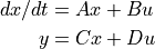
where is the input, is the output, and is the state. State space systems are usually created with the ss factory function.

Parameters

A, B, C, Darray_like

System matrices of the appropriate dimensions.

dtNone, True or float, optional

System timebase. 0 (default) indicates continuous time, True indicates discrete time with unspecified sampling time, positive number is discrete time with specified sampling time, None indicates unspecified timebase (either continuous or discrete time).

See also

ss, InputOutputSystem, NonlinearIOSystem

Notes

The main data members in the StateSpace class are the A, B, C, and D matrices. The class also keeps track of the number of states (i.e., the size of A).

A discrete-time system is created by specifying a nonzero ‘timebase’, dt when the system is constructed:

• dt = 0: continuous-time system (default)

• dt > 0: discrete-time system with sampling period dt

• dt = True: discrete time with unspecified sampling period

• dt = None: no timebase specified

Systems must have compatible timebases in order to be combined. A discrete-time system with unspecified sampling time (dt = True) can be combined with a system having a specified sampling time; the result will be a discrete-time system with the sample time of the other system. Similarly, a system with timebase None can be combined with a system having any timebase; the result will have the timebase of the other system. The default value of dt can be changed by changing the value of config.defaults['control.default_dt'].

A state space system is callable and returns the value of the transfer function evaluated at a point in the complex plane. See StateSpace.__call__ for a more detailed description.

Subsystems corresponding to selected input/output pairs can be created by indexing the state space system:

subsys = sys[output_spec, input_spec]

The input and output specifications can be single integers, lists of integers, or slices. In addition, the strings representing the names of the signals can be used and will be replaced with the equivalent signal offsets. The subsystem is created by truncating the inputs and outputs, but leaving the full set of system states.

StateSpace instances have support for IPython HTML/LaTeX output, intended for pretty-printing in Jupyter notebooks. The HTML/LaTeX output can be configured using config.defaults['statesp.latex_num_format'] and config.defaults['statesp.latex_repr_type']. The HTML/LaTeX output is tailored for MathJax, as used in Jupyter, and may look odd when typeset by non-MathJax LaTeX systems.

config.defaults['statesp.latex_num_format'] is a format string fragment, specifically the part of the format string after ‘{:’ used to convert floating-point numbers to strings. By default it is ‘.3g’.

config.defaults['statesp.latex_repr_type'] must either be ‘partitioned’ or ‘separate’. If ‘partitioned’, the A, B, C, D matrices are shown as a single, partitioned matrix; if ‘separate’, the matrices are shown separately.

Attributes

ninputs, noutputs, nstatesint

Number of input, output and state variables.

shapetuple

2-tuple of I/O system dimension, (noutputs, ninputs).

input_labels, output_labels, state_labelslist of str

Names for the input, output, and state variables.

namestring, optional

System name.

Attributes

A	Dynamics matrix.
B	Input matrix.
C	Output matrix.
D	Direct term.
dt	System timebase.
input_labels	List of labels for the input signals.
ninputs	Number of system inputs.
noutputs	Number of system outputs.
nstates	Number of system states.
output_labels	List of labels for the output signals.
repr_format	String representation format.
shape	2-tuple of I/O system dimension, (noutputs, ninputs).
state_labels	List of labels for the state signals.
states	Deprecated attribute; use nstates instead.

Methods

__call__	Evaluate system transfer function at point in complex plane.
append	Append a second model to the present model.
bandwidth	Evaluate bandwidth of an LTI system for a given dB drop.
bode_plot	Generate a Bode plot for the system.
copy	Make a copy of an input/output system.
damp	Natural frequency, damping ratio of system poles.
dcgain	Return the zero-frequency ("DC") gain.
dynamics	Compute the dynamics of the system.
feedback	Feedback interconnection between two LTI objects.
find_input	Find the index for an input given its name (None if not found).
find_inputs	Return list of indices matching input spec (None if not found).
find_output	Find the index for a output given its name (None if not found).
find_outputs	Return list of indices matching output spec (None if not found).
find_state	Find the index for a state given its name (None if not found).
find_states	Return list of indices matching state spec (None if not found).
forced_response	Generate the forced response for the system.
freqresp	(deprecated) Evaluate transfer function at complex frequencies.
frequency_response	Evaluate LTI system response at an array of frequencies.
horner	Evaluate value of transfer function using Horner's method.
impulse_response	Generate the impulse response for the system.
initial_response	Compute the initial condition response for a linear system.
isctime	Check to see if a system is a continuous-time system.
isdtime	Check to see if a system is a discrete-time system.
ispassive	Indicate if a linear time invariant (LTI) system is passive.
issiso	Check to see if a system is single input, single output.
lft	Return the linear fractional transformation.
linearize	Linearize an input/output system at a given state and input.
minreal	Remove unobservable and uncontrollable states.
nichols_plot	Generate a Nichols plot for the system.
nyquist_plot	Generate a Nyquist plot for the system.
output	Compute the output of the system.
poles	Compute the poles of a state space system.
returnScipySignalLTI	Return a list of a list of scipy.signal.lti objects.
sample	Convert a continuous-time system to discrete time.
set_inputs	Set the number/names of the system inputs.
set_outputs	Set the number/names of the system outputs.
set_states	Set the number/names of the system states.
slycot_laub	Laub's method to evaluate response at complex frequency.
step_response	Generate the step response for the system.
to_ss	Convert to state space representation.
to_tf	Convert to transfer function representation.
update_names	Update signal and system names for an I/O system.
zeros	Compute the zeros of a state space system.

A

Dynamics matrix.

B

Input matrix.

C

Output matrix.

D

Direct term.

__add__(other)

Add two LTI systems (parallel connection).

__call__(x, squeeze=None, warn_infinite=True)

Evaluate system transfer function at point in complex plane.

Returns the value of the system’s transfer function at a point x in the complex plane, where x is s for continuous-time systems and z for discrete-time systems.

See LTI.__call__ for details.

Examples

>>> G = ct.ss([[-1, -2], [3, -4]], [[5], [7]], [[6, 8]], [[9]])
>>> fresp = G(1j)  # evaluate at s = 1j

__getitem__(key)

Array style access

__mul__(other)

Multiply two LTI objects (serial connection).

__neg__()

Negate a state space system.

__pow__(other)

Power of a state space system

__radd__(other)

Right add two LTI systems (parallel connection).

__rmul__(other)

Right multiply two LTI objects (serial connection).

__rsub__(other)

Right subtract two LTI systems.

__rtruediv__(other)

Division by state space system

__sub__(other)

Subtract two LTI systems.

__truediv__(other)

Division of state space systems by TFs, FRDs, scalars, and arrays

append(other)

Append a second model to the present model.

The second model is converted to state-space if necessary, inputs and outputs are appended and their order is preserved.

Parameters

otherStateSpace or TransferFunction

System to be appended.

Returns

sysStateSpace

System model with other appended to self.

bandwidth(dbdrop=-3)

Evaluate bandwidth of an LTI system for a given dB drop.

Evaluate the first frequency that the response magnitude is lower than DC gain by dbdrop dB.

Parameters

dbdropfloat, optional

A strictly negative scalar in dB (default = -3) defines the amount of gain drop for deciding bandwidth.

Returns

bandwidthndarray

The first frequency (rad/time-unit) where the gain drops below dbdrop of the dc gain of the system, or nan if the system has infinite dc gain, inf if the gain does not drop for all frequency.

Raises

TypeError

If sys is not an SISO LTI instance.

ValueError

If dbdrop is not a negative scalar.

bode_plot(*args, **kwargs)

Generate a Bode plot for the system.

See bode_plot for more information.

copy(name=None, use_prefix_suffix=True)

Make a copy of an input/output system.

A copy of the system is made, with a new name. The name keyword can be used to specify a specific name for the system. If no name is given and use_prefix_suffix is True, the name is constructed by prepending config.defaults['iosys.duplicate_system_name_prefix'] and appending config.defaults['iosys.duplicate_system_name_suffix']. Otherwise, a generic system name of the form ‘sys[<id>]’ is used, where ‘<id>’ is based on an internal counter.

Parameters

namestr, optional

Name of the newly created system.

use_prefix_suffixbool, optional

If True and name is None, set the name of the new system to the name of the original system with prefix config.defaults['duplicate_system_name_prefix'] and suffix config.defaults['duplicate_system_name_suffix'].

Returns

InputOutputSystem

damp()

Natural frequency, damping ratio of system poles.

Returns

wnarray

Natural frequency for each system pole.

zetaarray

Damping ratio for each system pole.

polesarray

System pole locations.

dcgain(warn_infinite=False)

Return the zero-frequency (“DC”) gain.

The zero-frequency gain of a continuous-time state-space system is given by:

and of a discrete-time state-space system by:

Parameters

warn_infinitebool, optional

By default, don’t issue a warning message if the zero-frequency gain is infinite. Setting warn_infinite to generate the warning message.

Returns

gain(noutputs, ninputs) ndarray or scalar

Array or scalar value for SISO systems, depending on config.defaults['control.squeeze_frequency_response']. The value of the array elements or the scalar is either the zero-frequency (or DC) gain, or inf, if the frequency response is singular.

For real valued systems, the empty imaginary part of the complex zero-frequency response is discarded and a real array or scalar is returned.

dt

System timebase.

dynamics(t, x, u=None, params=None)

Compute the dynamics of the system.

Given input u and state x, returns the dynamics of the state-space system. If the system is continuous, returns the time derivative dx/dt

dx/dt = A x + B u

where A and B are the state-space matrices of the system. If the system is discrete time, returns the next value of x:

x[t+dt] = A x[t] + B u[t]

The inputs x and u must be of the correct length for the system.

The first argument t is ignored because StateSpace systems are time-invariant. It is included so that the dynamics can be passed to numerical integrators, such as scipy.integrate.solve_ivp and for consistency with InputOutputSystem models.

Parameters

tfloat (ignored)

Time.

xarray_like

Current state.

uarray_like (optional)

Input, zero if omitted.

Returns

dx/dt or x[t+dt]ndarray

feedback(other=1, sign=-1)

Feedback interconnection between two LTI objects.

Parameters

otherInputOutputSystem

System in the feedback path.

signfloat, optional

Gain to use in feedback path. Defaults to -1.

find_input(name)

Find the index for an input given its name (None if not found).

Parameters

namestr

Signal name for the desired input.

Returns

int

Index of the named input.

find_inputs(name_list)

Return list of indices matching input spec (None if not found).

Parameters

name_liststr or list of str

List of signal specifications for the desired inputs. A signal can be described by its name or by a slice-like description of the form ‘start:end` where ‘start’ and ‘end’ are signal names. If either is omitted, it is taken as the first or last signal, respectively.

Returns

list of int

List of indices for the specified inputs.

find_output(name)

Find the index for a output given its name (None if not found).

Parameters

namestr

Signal name for the desired output.

Returns

int

Index of the named output.

find_outputs(name_list)

Return list of indices matching output spec (None if not found).

Parameters

name_liststr or list of str

List of signal specifications for the desired outputs. A signal can be described by its name or by a slice-like description of the form ‘start:end` where ‘start’ and ‘end’ are signal names. If either is omitted, it is taken as the first or last signal, respectively.

Returns

list of int

List of indices for the specified outputs.

find_state(name)

Find the index for a state given its name (None if not found).

Parameters

namestr

Signal name for the desired state.

Returns

int

Index of the named state.

find_states(name_list)

Return list of indices matching state spec (None if not found).

Parameters

name_liststr or list of str

List of signal specifications for the desired states. A signal can be described by its name or by a slice-like description of the form ‘start:end` where ‘start’ and ‘end’ are signal names. If either is omitted, it is taken as the first or last signal, respectively.

Returns

list of int

List of indices for the specified states..

forced_response(*args, **kwargs)

Generate the forced response for the system.

See forced_response for more information.

freqresp(omega)

(deprecated) Evaluate transfer function at complex frequencies.

frequency_response(omega=None, squeeze=None)

Evaluate LTI system response at an array of frequencies.

See frequency_response for more detailed information.

horner(x, warn_infinite=True)

Evaluate value of transfer function using Horner’s method.

Evaluates sys(x) where x is a complex number s for continuous-time systems and z for discrete-time systems. Expects inputs and outputs to be formatted correctly. Use sys(x) for a more user-friendly interface.

Parameters

xcomplex

Complex frequency at which the transfer function is evaluated.

warn_infinitebool, optional

If True (default), generate a warning if x is a pole.

Returns

complex

Notes

Attempts to use Laub’s method from Slycot library, with a fall-back to Python code.

impulse_response(*args, **kwargs)

Generate the impulse response for the system.

See impulse_response for more information.

initial_response(timepts=None, initial_state=0, output_indices=None, timepts_num=None, params=None, transpose=False, return_states=False, squeeze=None, **kwargs)

Compute the initial condition response for a linear system.

If the system has multiple outputs (MIMO), optionally, one output may be selected. If no selection is made for the output, all outputs are given.

For information on the shape of parameters T, X0 and return values T, yout, see Time series data conventions.

Parameters

sysdataI/O system or list of I/O systems

I/O system(s) for which initial response is computed.

timepts (or T)array_like or float, optional

Time vector, or simulation time duration if a number (time vector is auto-computed if not given; see step_response for more detail).

initial_state (or X0)array_like or float, optional

Initial condition (default = 0). Numbers are converted to constant arrays with the correct shape.

output_indices (or output)int

Index of the output that will be used in this simulation. Set to None to not trim outputs.

timepts_num (or T_num)int, optional

Number of time steps to use in simulation if timepts is not provided as an array (auto-computed if not given); ignored if the system is discrete time.

paramsdict, optional

If system is a nonlinear I/O system, set parameter values.

transposebool, optional

If True, transpose all input and output arrays (for backward compatibility with MATLAB and scipy.signal.lsim). Default value is False.

return_states (or return_x)bool, optional

If True, return the state vector when assigning to a tuple (default = False). See forced_response for more details.

squeezebool, optional

By default, if a system is single-input, single-output (SISO) then the output response is returned as a 1D array (indexed by time). If squeeze = True, remove single-dimensional entries from the shape of the output even if the system is not SISO. If squeeze = False, keep the output as a 2D array (indexed by the output number and time) even if the system is SISO. The default value can be set using config.defaults['control.squeeze_time_response'].

Returns

resultsTimeResponseData or TimeResponseList

Time response represented as a TimeResponseData object or list of TimeResponseData objects. See forced_response for additional information.

See also

forced_response, impulse_response, step_response

Notes

This function uses the forced_response function with the input set to zero.

Examples

>>> G = ct.rss(4)
>>> T, yout = ct.initial_response(G)

property input_labels

List of labels for the input signals.

isctime(strict=False)

Check to see if a system is a continuous-time system.

Parameters

strictbool, optional

If strict is True, make sure that timebase is not None. Default is False.

isdtime(strict=False)

Check to see if a system is a discrete-time system.

Parameters

strictbool, optional

If strict is True, make sure that timebase is not None. Default is False.

ispassive()

Indicate if a linear time invariant (LTI) system is passive.

See ispassive for details.

issiso()

Check to see if a system is single input, single output.

lft(other, nu=-1, ny=-1)

Return the linear fractional transformation.

A definition of the LFT operator can be found in Appendix A.7, page 512 in [1]. An alternative definition can be found here: https://www.mathworks.com/help/control/ref/lft.html

Parameters

otherStateSpace

The lower LTI system.

nyint, optional

Dimension of (plant) measurement output.

nuint, optional

Dimension of (plant) control input.

Returns

StateSpace

References

1

S. Skogestad, Multivariable Feedback Control. Second edition, 2005.

linearize(x0, u0=None, t=0, params=None, eps=1e-06, copy_names=False, **kwargs)

Linearize an input/output system at a given state and input.

Return the linearization of an input/output system at a given operating point (or state and input value) as a StateSpace system. See linearize for complete documentation.

minreal(tol=0.0)

Remove unobservable and uncontrollable states.

Calculate a minimal realization for a state space system, removing all unobservable and/or uncontrollable states.

Parameters

tolfloat

Tolerance for determining whether states are unobservable or uncontrollable.

nichols_plot(*args, **kwargs)

Generate a Nichols plot for the system.

See nichols_plot for more information.

ninputs

Number of system inputs.

noutputs

Number of system outputs.

nstates

Number of system states.

nyquist_plot(*args, **kwargs)

Generate a Nyquist plot for the system.

See nyquist_plot for more information.

output(t, x, u=None, params=None)

Compute the output of the system.

Given input u and state x, returns the output y of the state-space system:

y = C x + D u

where A and B are the state-space matrices of the system.

The first argument t is ignored because StateSpace systems are time-invariant. It is included so that the dynamics can be passed to most numerical integrators, such as SciPy’s integrate.solve_ivp and for consistency with InputOutputSystem models.

The inputs x and u must be of the correct length for the system.

Parameters

tfloat (ignored)

Time.

xarray_like

Current state.

uarray_like (optional)

Input (zero if omitted).

Returns

yndarray

property output_labels

List of labels for the output signals.

poles()

Compute the poles of a state space system.

property repr_format

String representation format.

Format used in creating the representation for the system:

• ‘info’ : <IOSystemType sysname: [inputs] -> [outputs]>

• ‘eval’ : system specific, loadable representation

• ‘latex’ : HTML/LaTeX representation of the object

The default representation for an input/output is set to ‘eval’. This value can be changed for an individual system by setting the repr_format parameter when the system is created or by setting the repr_format property after system creation. Set config.defaults['iosys.repr_format'] to change for all I/O systems or use the repr_format parameter/attribute for a single system.

returnScipySignalLTI(strict=True)

Return a list of a list of scipy.signal.lti objects.

For instance,

>>> out = ssobject.returnScipySignalLTI()               
>>> out[3][5]                                           

is a scipy.signal.lti object corresponding to the transfer function from the 6th input to the 4th output.

Parameters

strictbool, optional

True (default):

The timebase ssobject.dt cannot be None; it must be continuous (0) or discrete (True or > 0).

False:

If ssobject.dt is None, continuous-time scipy.signal.lti objects are returned.

Returns

outlist of list of scipy.signal.StateSpace

Continuous time (inheriting from scipy.signal.lti) or discrete time (inheriting from scipy.signal.dlti) SISO objects.

sample(Ts, method='zoh', alpha=None, prewarp_frequency=None, name=None, copy_names=True, **kwargs)

Convert a continuous-time system to discrete time.

Creates a discrete-time system from a continuous-time system by sampling. Multiple methods of conversion are supported.

Parameters

Tsfloat

Sampling period.

method{‘gbt’, ‘bilinear’, ‘euler’, ‘backward_diff’, ‘zoh’}

Method to use for sampling:

• ‘gbt’: generalized bilinear transformation

• ‘backward_diff’: Backwards difference (‘gbt’ with alpha=1.0)

• ‘bilinear’ (or ‘tustin’): Tustin’s approximation (‘gbt’ with alpha=0.5)

• ‘euler’: Euler (or forward difference) method (‘gbt’ with alpha=0)

• ‘zoh’: zero-order hold (default)

alphafloat within [0, 1]

The generalized bilinear transformation weighting parameter, which should only be specified with method=’gbt’, and is ignored otherwise.

prewarp_frequencyfloat within [0, infinity)

The frequency [rad/s] at which to match with the input continuous-time system’s magnitude and phase (the gain = 1 crossover frequency, for example). Should only be specified with method = ‘bilinear’ or ‘gbt’ with alpha = 0.5 and ignored otherwise.

namestring, optional

Set the name of the sampled system. If not specified and if copy_names is False, a generic name ‘sys[id]’ is generated with a unique integer id. If copy_names is True, the new system name is determined by adding the prefix and suffix strings in config.defaults['iosys.sampled_system_name_prefix'] and config.defaults['iosys.sampled_system_name_suffix'], with the default being to add the suffix ‘$sampled’.

copy_namesbool, Optional

If True, copy the names of the input signals, output signals, and states to the sampled system.

Returns

sysdStateSpace

Discrete-time system, with sampling rate Ts.

Other Parameters

inputsint, list of str or None, optional

Description of the system inputs. If not specified, the original system inputs are used. See InputOutputSystem for more information.

outputsint, list of str or None, optional

Description of the system outputs. Same format as inputs.

statesint, list of str, or None, optional

Description of the system states. Same format as inputs.

Notes

Uses scipy.signal.cont2discrete.

Examples

>>> G = ct.ss(0, 1, 1, 0)
>>> sysd = G.sample(0.5, method='bilinear')

set_inputs(inputs, prefix='u')

Set the number/names of the system inputs.

Parameters

inputsint, list of str, or None

Description of the system inputs. This can be given as an integer count or as a list of strings that name the individual signals. If an integer count is specified, the names of the signal will be of the form ‘u[i]’ (where the prefix ‘u’ can be changed using the optional prefix parameter).

prefixstring, optional

If inputs is an integer, create the names of the states using the given prefix (default = ‘u’). The names of the input will be of the form ‘prefix[i]’.

set_outputs(outputs, prefix='y')

Set the number/names of the system outputs.

Parameters

outputsint, list of str, or None

Description of the system outputs. This can be given as an integer count or as a list of strings that name the individual signals. If an integer count is specified, the names of the signal will be of the form ‘y[i]’ (where the prefix ‘y’ can be changed using the optional prefix parameter).

prefixstring, optional

If outputs is an integer, create the names of the states using the given prefix (default = ‘y’). The names of the input will be of the form ‘prefix[i]’.

set_states(states, prefix='x')

Set the number/names of the system states.

Parameters

statesint, list of str, or None

Description of the system states. This can be given as an integer count or as a list of strings that name the individual signals. If an integer count is specified, the names of the signal will be of the form ‘x[i]’ (where the prefix ‘x’ can be changed using the optional prefix parameter).

prefixstring, optional

If states is an integer, create the names of the states using the given prefix (default = ‘x’). The names of the input will be of the form ‘prefix[i]’.

property shape

2-tuple of I/O system dimension, (noutputs, ninputs).

slycot_laub(x)

Laub’s method to evaluate response at complex frequency.

Evaluate transfer function at complex frequency using Laub’s method from Slycot. Expects inputs and outputs to be formatted correctly. Use sys(x) for a more user-friendly interface.

Parameters

xcomplex array_like or complex

Complex frequency.

Returns

output(number_outputs, number_inputs, len(x)) complex ndarray

Frequency response.

property state_labels

List of labels for the state signals.

property states

Deprecated attribute; use nstates instead.

The state attribute was used to store the number of states for : a state space system. It is no longer used. If you need to access the number of states, use nstates.

step_response(*args, **kwargs)

Generate the step response for the system.

See step_response for more information.

to_ss(*args, **kwargs)

Convert to state space representation.

See ss for details.

to_tf(*args, **kwargs)

Convert to transfer function representation.

See tf for details.

update_names([name, inputs, outputs, states])

Update signal and system names for an I/O system.

Parameters

namestr, optional

New system name.

inputslist of str, int, or None, optional

List of strings that name the individual input signals. If given as an integer or None, signal names default to the form ‘u[i]’. See InputOutputSystem for more information.

outputslist of str, int, or None, optional

Description of output signals; defaults to ‘y[i]’.

statesint, list of str, int, or None, optional

Description of system states; defaults to ‘x[i]’.

input_prefixstring, optional

Set the prefix for input signals. Default = ‘u’.

output_prefixstring, optional

Set the prefix for output signals. Default = ‘y’.

state_prefixstring, optional

Set the prefix for state signals. Default = ‘x’.

zeros()

Compute the zeros of a state space system.