6. Interconnected I/O Systems
Input/output systems can be interconnected in a variety of ways,
including operator overloading, block diagram algebra functions, and
using the interconnect() function to build a hierarchical system
description. This chapter provides more detailed information on
operator overloading and block diagram algebra, as well as a
description of the InterconnectedSystem class, which can be
created using the interconnect() function.
6.1. Operator Overloading
The following operators are defined to operate between I/O systems:
Operation |
Description |
Equivalent command |
|---|---|---|
|
Add the outputs of two systems receiving the same input |
|
|
Connect output(s) of sys2 to input(s) of sys1 |
|
|
Multiply the output(s) of the system by -1 |
|
|
Divide one SISO transfer function by another |
N/A |
|
Multiply a transfer function by itself |
N/A |
If either of the systems is a scalar or an array of appropriate dimension, then the appropriate scalar or matrix operation is performed. In addition, if a SISO system is combined with a MIMO system, the SISO system will be broadcast to the appropriate shape.
Systems of different types can be combined using these operations, with the following rules:
If both systems can be converted into the type of the other, the leftmost system determines the type of the output.
If only one system can be converted into the other, then the more general system determines the type of the output. In particular:
State space and transfer function systems can be converted to nonlinear systems.
Linear systems can be converted to frequency response data (FRD) systems, using the frequencies of the FRD system.
FRD systems can only be combined with FRD systems, constants, and arrays.
6.2. Block Diagram Algebra
Block diagram algebra is implemented using the following functions:
|
Series connection of I/O systems. |
|
Parallel connection of I/O systems. |
|
Feedback interconnection between two I/O systems. |
|
Return the negative of a system. |
|
Group LTI models by appending their inputs and outputs. |
The feedback() function implements a standard feedback
interconnection between two systems, as illustrated in the following
diagram:

By default a gain of -1 is applied at the output of the second system, so the dynamics illustrate above can be created using the command
Gyu = ct.feedback(G1, G2)
An optional gain parameter can be used to change the sign of the gain.
The feedback() function is also implemented via the
LTI.feedback() method, so if G1 is an input/output system then
the following command will also work:
Gyu = G1.feedback(G2)
All block diagram algebra functions allow the name of the system and
labels for signals to be specified using the usual name, inputs,
and outputs keywords, as described in the InputOutputSystem
class. For state space systems, the labels for the states can also be
given, but caution should be used since the order of states in the
combined system is not guaranteed.
6.3. Signal-Based Interconnection
More complex input/output systems can be constructed by using the
interconnect() function, which allows a collection of
input/output subsystems to be combined with internal connections
between the subsystems and a set of overall system inputs and outputs
that link to the subsystems. For example, the closed loop dynamics of
a feedback control system using the standard names and labels for
inputs and outputs could be constructed using the command
clsys = ct.interconnect(
    [plant, controller], name='system',
    connections=[
        ['controller.u', '-plant.y'],
        ['plant.u', 'controller.y']],
    inplist=['controller.u'], inputs='r',
    outlist=['plant.y'], outputs='y')
The remainder of this section provides a detailed description of the
operation of the interconnect() function.
Illustrative example
To illustrate the use of the interconnect() function, we create a
model for a predator/prey system, following the notation and parameter
values in Feedback Systems.
We begin by defining the dynamics of the system:
import matplotlib.pyplot as plt
import numpy as np
import control as ct

def predprey_rhs(t, x, u, params):
    # Parameter setup
    a = params.get('a', 3.2)
    b = params.get('b', 0.6)
    c = params.get('c', 50.)
    d = params.get('d', 0.56)
    k = params.get('k', 125)
    r = params.get('r', 1.6)

    # Map the states into local variable names
    H = x[0]
    L = x[1]

    # Compute the control action (only allow addition of food)
    u_0 = u[0] if u[0] > 0 else 0

    # Compute the discrete updates
    dH = (r + u_0) * H * (1 - H/k) - (a * H * L)/(c + H)
    dL = b * (a * H *  L)/(c + H) - d * L

    return np.array([dH, dL])
We now create an input/output system using these dynamics:
predprey = ct.nlsys(
    predprey_rhs, None, inputs=['u'], outputs=['Hares', 'Lynxes'],
    states=['H', 'L'], name='predprey')
Note that since we have not specified an output function, the entire state will be used as the output of the system.
The predprey system can now be simulated to obtain the open loop
dynamics of the system:
X0 = [25, 20]                      # Initial H, L
timepts = np.linspace(0, 70, 500)  # Simulation 70 years of time

# Simulate the system and plots the results
resp = ct.input_output_response(predprey, timepts, 0, X0)
resp.plot(plot_inputs=False, overlay_signals=True, legend_loc='upper left')

We can also create a feedback controller to stabilize a desired population of the system. We begin by finding the (unstable) equilibrium point for the system and computing the linearization about that point.
xeq, ueq = ct.find_operating_point(predprey, X0, 0)
lin_predprey = ct.linearize(predprey, xeq, ueq)
We next compute a controller that stabilizes the equilibrium point using eigenvalue placement and computing the feedforward gain using the number of lynxes as the desired output (following Feedback Systems, Example 7.5):
K = ct.place(lin_predprey.A, lin_predprey.B, [-0.1, -0.2])
A, B = lin_predprey.A, lin_predprey.B
C = np.array([[0, 1]])                # regulated output = number of lynxes
kf = -1/(C @ np.linalg.inv(A - B @ K) @ B)
To construct the control law, we build a simple input/output system that
applies a corrective input based on deviations from the equilibrium point.
This system has no dynamics, since it is a static (affine) map, and can
constructed using nlsys() with no update function:
def output(t, x, u, params):
    Ld, x, ye = u[0], u[1:], xeq[1]
    return ueq - K @ (x - xeq) + kf * (Ld - ye)

controller = ct.nlsys(
    None, output,
    inputs=['Ld', 'H', 'L'], outputs=1, name='control')
The input to the controller is u, consisting of the desired lynx
population followed by the vector of hare and lynx populations.
To connect the controller to the predatory-prey model, we use the
interconnect() function:
closed = ct.interconnect(
  [predprey, controller],     # systems
  connections=[
    ['predprey.u', 'control.y[0]'],
    ['control.H',  'predprey.Hares'],
    ['control.L',  'predprey.Lynxes']
  ],
  inplist=['control.Ld'], inputs='Ld',
  outlist=['predprey.Hares', 'predprey.Lynxes', 'control.y[0]'],
  outputs=['Hares', 'Lynxes', 'u0'], name='closed loop'
)
Finally, we simulate the closed loop system:
# Simulate the system
Ld = 30
resp = ct.input_output_response(
    closed, timepts, inputs=Ld, initial_state=[15, 20])
cplt = resp.plot(
    plot_inputs=False, overlay_signals=True, legend_loc='upper left')
cplt.axes[0, 0].axhline(Ld, linestyle='--', color='black')

This example shows the standard operations that would be used to build up an interconnected nonlinear system. The I/O systems module has a number of other features that can be used to simplify the creation and use of interconnected input/output systems.
Summing junction
The summing_junction() function can be used to create an
input/output system that takes the sum of an arbitrary number of inputs. For
example, to create an input/output system that takes the sum of three inputs,
use the command
sumblk = ct.summing_junction(3)
By default, the name of the inputs will be of the form ‘u[i]’ and the output will be ‘y’. This can be changed by giving an explicit list of names:
sumblk = ct.summing_junction(inputs=['a', 'b', 'c'], output='d')
A more typical usage would be to define an input/output system that compares a reference signal to the output of the process and computes the error:
sumblk = ct.summing_junction(inputs=['r', '-y'], output='e')
Note the use of the minus sign as a means of setting the sign of the input ‘y’ to be negative instead of positive.
It is also possible to define “vector” summing blocks that take multi-dimensional inputs and produce a multi-dimensional output. For example, the command
sumblk = ct.summing_junction(inputs=['r', '-y'], output='e', dimension=2)
will produce an input/output block that implements e[0] = r[0] - y[0] and
e[1] = r[1] - y[1].
Automatic connections using signal names
The interconnect() function allows the interconnection of
multiple systems by using signal names of the form ‘sys.signal’. In many
situations, it can be cumbersome to explicitly connect all of the appropriate
inputs and outputs. As an alternative, if the connections keyword is
omitted, the interconnect() function will connect all signals
of the same name to each other. This can allow for simplified methods of
interconnecting systems, especially when combined with the
summing_junction() function. For example, the following code
will create a unity gain, negative feedback system:
P = ct.tf([1], [1, 0], inputs='u', outputs='y')
C = ct.tf([10], [1, 1], inputs='e', outputs='u')
sumblk = ct.summing_junction(inputs=['r', '-y'], output='e')
T = ct.interconnect([P, C, sumblk], inplist='r', outlist='y')
If a signal name appears in multiple outputs then that signal will be summed
when it is interconnected. Similarly, if a signal name appears in multiple
inputs then all systems using that signal name will receive the same input.
The interconnect() function will generate an error if a signal
listed in inplist or outlist (corresponding to the inputs and outputs
of the interconnected system) is not found, but inputs and outputs of
individual systems that are not connected to other systems are left
unconnected (so be careful!).
Vector element processing
Several I/O system commands perform processing of vector elements (such as initial states or input vectors) and broadcast these to the proper shape.
For static elements, such as the initial state in a simulation or the nominal state and input for a linearization, the following processing is done:
Scalars are automatically converted to a vector of the appropriate size consisting of the scalar value. This is commonly used when specifying the origin (‘0’) or a step input (‘1’).
Lists of values are concatenated into a single vector. This is often used when you have an interconnected system and you need to specify the initial condition or input value for each subsystem (e.g., [X1eq, X2eq, …]).
Vector elements are zero padded to the required length. If you specify only a portion of the values for states or inputs, the remaining values are taken as zero. (If the final element in the given vector is non-zero, a warning is issued.)
Similar processing is done for input time series, used for the
input_output_response() and
forced_response() commands, with the following
additional feature:
Time series elements are broadcast to match the number of time points specified. If a list of time series and static elements are given (as a list), static elements are broadcast to the proper number of time points, and the overall list of elements concatenated to provide the full input vector.
As an example, suppose we have an interconnected system consisting of three subsystems, a controlled process, an estimator, and a (static) controller:
proc = ct.nlsys(...,
    states=2, inputs=['u1', 'u2', 'd'], outputs='y')
estim = ct.nlsys(...,
    states=2, inputs='y', outputs=['xhat[0]', 'xhat[1]')
ctrl = ct.nlsys(...,
    states=0, inputs=['r', 'xhat[0]', 'xhat[1]'], outputs=['u1', 'u2'])

clsys = ct.interconnect(
    [proc, estim, ctrl], inputs=['r', 'd'], outputs=['y', 'u1', 'u2'])
To linearize the system around the origin, we can utilize the scalar processing feature of vector elements:
P = proc.linearize(0, 0)
In this command, the states and the inputs are broadcast to the size of the state and input vectors, respectively.
If we want to linearize the closed loop system around a process state
x0 (with two elements) and an estimator state 0 (for both states),
we can use the list processing feature:
H = clsys.linearize([x0, 0], 0)
Note that this also utilizes the zero-padding functionality, since the
second argument in the list [x0, 0] is a scalar and so the vector
[x0, 0] only has three elements instead of the required four.
To run an input/output simulation with a sinusoidal signal for the first input, a constant for the second input, and no external disturbance, we can use the list processing feature combined with time series broadcasting:
timepts = np.linspace(0, 10)
u1 = np.sin(timepts)
u2 = 1
resp = ct.input_output_response(clsys, timepts, [u1, u2, 0])
In this command, the second and third arguments will be broadcast to match the number of time points.
Advanced specification of signal names
In addition to manual specification of signal names and automatic
connection of signals with the same name, the
interconnect() has a variety of other mechanisms
available for specifying signal names. The following forms are
recognized for the connections, inplist, and outlist
parameters:
(subsys, index, gain)             tuple form with integer indices
('sysname', 'signal', gain)       tuple form with name lookup
'sysname.signal[i]'               string form (gain = 1)
'-sysname.signal[i]'              set gain to -1
(subsys, [i1, ..., iN], gain)     signals with indices i1, ..., in
'sysname.signal[i:j]'             range of signal names, i through j-1
'sysname'                         all input or outputs of system
'signal'                          all matching signals (in any subsystem)
For tuple forms, mixed specifications using integer indices and strings are possible.
For the index range form sysname.signal[i:j], if either i or j
is not specified, then it defaults to the minimum or maximum value of
the signal range. Note that despite the similarity to slice notation,
negative indices and step specifications are not supported.
Using these various forms can simplify the specification of interconnections. For example, consider a process with inputs ‘u’ and ‘v’, each of dimension 2, and two outputs ‘w’ and ‘y’, each of dimension 2:
P = ct.ss(
    np.diag([-1, -2, -3, -4]), np.eye(4), np.eye(4), 0, name='P',
    inputs=['u[0]', 'u[1]', 'v[0]', 'v[1]'],
    outputs=['y[0]', 'y[1]', 'z[0]', 'z[1]'])
Suppose we construct a controller with 2 inputs and 2 outputs that takes the (2-dimensional) error ‘e’ and outputs and control signal ‘u’:
C = ct.ss(
    [], [], [], [[3, 0], [0, 4]],
    name='C', input_prefix='e', output_prefix='u')
Finally, we include a summing block that will take the difference between the reference input ‘r’ and the measured output ‘y’:
sumblk = ct.summing_junction(
  inputs=['r', '-y'], outputs='e', dimension=2, name='sum')
The closed loop system should close the loop around the process outputs ‘y’ and inputs ‘u’, leaving the process inputs ‘v’ and outputs ‘w’, as well as the reference input ‘r’. We would like the output of the closed loop system to consist of all system outputs ‘y’ and ‘z’, as well as the controller input ‘u’.
This collection of systems can be combined in a variety of ways. The most explicit would specify every signal:
clsys1 = ct.interconnect(
  [C, P, sumblk],
  connections=[
    ['P.u[0]', 'C.u[0]'], ['P.u[1]', 'C.u[1]'],
    ['C.e[0]', 'sum.e[0]'], ['C.e[1]', 'sum.e[1]'],
    ['sum.y[0]', 'P.y[0]'], ['sum.y[1]', 'P.y[1]'],
  ],
  inplist=['sum.r[0]', 'sum.r[1]', 'P.v[0]', 'P.v[1]'],
  outlist=['P.y[0]', 'P.y[1]', 'P.z[0]', 'P.z[1]', 'C.u[0]', 'C.u[1]']
)
This connections can be simplified using signal ranges:
clsys2 = ct.interconnect(
  [C, P, sumblk],
  connections=[
    ['P.u[0:2]', 'C.u[0:2]'],
    ['C.e[0:2]', 'sum.e[0:2]'],
    ['sum.y[0:2]', 'P.y[0:2]']
  ],
  inplist=['sum.r[0:2]', 'P.v[0:2]'],
  outlist=['P.y[0:2]', 'P.z[0:2]', 'C.u[0:2]']
)
An even simpler form can be used by omitting the range specification when all signals with the same prefix are used:
clsys3 = ct.interconnect(
  [C, P, sumblk],
  connections=[['P.u', 'C.u'], ['C.e', 'sum.e'], ['sum.y', 'P.y']],
  inplist=['sum.r', 'P.v'], outlist=['P.y', 'P.z', 'C.u']
)
A further simplification is possible when all of the inputs or outputs of an individual system are used in a given specification:
clsys4 = ct.interconnect(
  [C, P, sumblk], name='clsys4',
  connections=[['P.u', 'C'], ['C', 'sum'], ['sum.y', 'P.y']],
  inplist=['sum.r', 'P.v'], outlist=['P', 'C.u']
)
And finally, since we have named the signals throughout the system in a
consistent way, we could let interconnect() do all of the
work:
clsys5 = ct.interconnect(
  [C, P, sumblk], inplist=['sum.r', 'P.v'], outlist=['P', 'C.u']
)
Various other simplifications are possible, but it can sometimes be
complicated to debug error message when things go wrong. Setting
debug = True when calling interconnect() prints out
information about how the arguments are processed that may be helpful
in understanding what is going wrong.
If the system is constructed successfully but the system does not seem
to behave correctly, the print function can be used to show the
interconnections and outputs:
>>> print(clsys4)
<LinearICSystem>: clsys4
Inputs (4): ['u[0]', 'u[1]', 'u[2]', 'u[3]']
Outputs (6): ['y[0]', 'y[1]', 'y[2]', 'y[3]', 'y[4]', 'y[5]']
States (4): ['P_x[0]', 'P_x[1]', 'P_x[2]', 'P_x[3]']

Subsystems (3):
 * <StateSpace C: ['e[0]', 'e[1]'] -> ['u[0]', 'u[1]'], dt=None>
 * <StateSpace P: ['u[0]', 'u[1]', 'v[0]', 'v[1]'] -> ['y[0]', 'y[1]', 'z[0]',
    'z[1]']>
 * <StateSpace sum: ['r[0]', 'r[1]', 'y[0]', 'y[1]'] -> ['e[0]', 'e[1]'],
    dt=None>

Connections:
 * C.e[0] <- sum.e[0]
 * C.e[1] <- sum.e[1]
 * P.u[0] <- C.u[0]
 * P.u[1] <- C.u[1]
 * P.v[0] <- u[2]
 * P.v[1] <- u[3]
 * sum.r[0] <- u[0]
 * sum.r[1] <- u[1]
 * sum.y[0] <- P.y[0]
 * sum.y[1] <- P.y[1]

Outputs:
 * y[0] <- P.y[0]
 * y[1] <- P.y[1]
 * y[2] <- P.z[0]
 * y[3] <- P.z[1]
 * y[4] <- C.u[0]
 * y[5] <- C.u[1]

A = [[-4.  0.  0.  0.]
     [ 0. -6.  0.  0.]
     [ 0.  0. -3.  0.]
     [ 0.  0.  0. -4.]]

B = [[3. 0. 0. 0.]
     [0. 4. 0. 0.]
     [0. 0. 1. 0.]
     [0. 0. 0. 1.]]

C = [[ 1.  0.  0.  0.]
     [ 0.  1.  0.  0.]
     [ 0.  0.  1.  0.]
     [ 0.  0.  0.  1.]
     [-3.  0.  0.  0.]
     [ 0. -4.  0.  0.]]

D = [[0. 0. 0. 0.]
     [0. 0. 0. 0.]
     [0. 0. 0. 0.]
     [0. 0. 0. 0.]
     [3. 0. 0. 0.]
     [0. 4. 0. 0.]]
6.4. Automated creation of state feedback systems
A common architecture in state space feedback control is to use a linear control law to stabilize a system around a trajectory. The python-control package can create input/output systems that help implement this architecture.
Standard design patterns
The create_statefbk_iosystem() function can be used to create an
I/O system consisting of a state feedback gain (with optional integral
action and gain scheduling) and an estimator. A basic state feedback
controller of the form
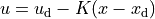
can be created with the command:
ctrl, clsys = ct.create_statefbk_iosystem(sys, K)
where sys is the process dynamics and K is the state feedback gain
(e.g., from LQR). The function returns the controller ctrl and the
closed loop systems clsys, both as I/O systems. The input to the
controller is the vector of desired states  , desired
inputs
, desired
inputs  , and system states
  .
.
If an InputOutputSystem is passed instead of the gain K, the error
e = x - xd is passed to the system and the output is used as the
feedback compensation term.
The above design pattern is referred to as the “trajectory generation”
(‘trajgen’) pattern, since it assumes that the input to the controller is a
feasible trajectory  . Alternatively, a
controller using the “reference gain” pattern can be created, which
implements a state feedback controller of the form
. Alternatively, a
controller using the “reference gain” pattern can be created, which
implements a state feedback controller of the form
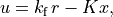
where  is the reference input and
  is the
feedforward gain (normally chosen so that the steady state output
is the
feedforward gain (normally chosen so that the steady state output
 will be equal to ).
A reference gain controller can be created with the command:
ctrl, clsys = ct.create_statefbk_iosystem(
    sys, K, kf, feedfwd_pattern='refgain')
This reference gain design pattern is described in more detail in Feedback Systems, Section 7.2 (Stabilization by State Feedback) and the trajectory generation design pattern is described in Section 8.5 (State Space Controller Design).
Adding state estimation
If the full system state is not available, the output of a state estimator can be used to construct the controller using the command:
ctrl, clsys = ct.create_statefbk_iosystem(sys, K, estimator=estim)
where estim is a state estimator I/O system. The controller will
have the same form as above, but with the system state
replaced by the estimated state  (output of
 estim).
The closed loop controller will include both the state feedback and
the estimator.
An estimator for a linear system should use the process inputs
 and outputs
  to generate an estimate
of the process state. An optimal estimator (Kalman) filter can be
constructed using the
to generate an estimate
of the process state. An optimal estimator (Kalman) filter can be
constructed using the create_estimator_iosystem() command:
estim = ct.create_estimator_iosystem(sys, QN, RN)
where QN is covariance matrix for the process disturbances (assumed
by default to enter at the process inputs) and RN is the covariance
matrix for the measurement noise.
As an example, consider a simple double integrator linear system with an LQR controller:
# System
sys = ct.ss([[0, 1], [0, 0]], [[0], [1]], [[1, 0]], 0, name='sys')

# Controller
K, _, _ = ct.lqr(sys, np.eye(2), np.eye(1))
We construct an estimator for the system assuming disturbance and noise intensity of 0.01:
# Estimator
estim = ct.create_estimator_iosystem(sys, 0.01, 0.01, name='estim')
resulting in the following dynamics:
>>> print(estim)
<NonlinearIOSystem>: estim
Inputs (2): ['y[0]', 'u[0]']
Outputs (2): ['xhat[0]', 'xhat[1]']
States (6): ['xhat[0]', 'xhat[1]', 'P[0,0]', 'P[0,1]', 'P[1,0]', 'P[1,1]']

Update: <function create_estimator_iosystem.<locals>._estim_update at 0x...>
Output: <function create_estimator_iosystem.<locals>._estim_output at 0x...>
The estimator is a nonlinear system with states consisting of the
estimates of the process states () and the entries of
the covariance of the state error ( ). The estimator dynamics
are given by
). The estimator dynamics
are given by

where  is the estimator gain and
  is the mapping
from disturbance signals to the state dynamics (see
is the mapping
from disturbance signals to the state dynamics (see
create_estimator_iosystem and Optimization-Based Control, Chapter 6 [Kalman Filtering] for more
detailed information).
We can now create the entire closed loop system using the estimated state:
# Estimation-based controller
ctrl, clsys = ct.create_statefbk_iosystem(
    sys, K, estimator=estim, name='ctrl')
The resulting controller is given by
>>> print(ctrl)
<StateSpace>: ctrl
Inputs (5): ['xd[0]', 'xd[1]', 'ud[0]', 'xhat[0]', 'xhat[1]']
Outputs (1): ['u[0]']
States (0): []

A = []

B = []

C = []

D = [[ 1.          1.73205081  1.         -1.         -1.73205081]]
Note that controller input signals have automatically been named to match the estimator output signals. The full closed loop system is given by
>>> print(clsys)
<InterconnectedSystem>: sys_ctrl
Inputs (3): ['xd[0]', 'xd[1]', 'ud[0]']
Outputs (2): ['y[0]', 'u[0]']
States (8): ['sys_x[0]', 'sys_x[1]', 'estim_xhat[0]', 'estim_xhat[1]', 'estim_P[0,0]', 'estim_P[0,1]', 'estim_P[1,0]', 'estim_P[1,1]']

Subsystems (3):
 * <StateSpace sys: ['u[0]'] -> ['y[0]']>
 * <StateSpace ctrl: ['xd[0]', 'xd[1]', 'ud[0]', 'xhat[0]', 'xhat[1]'] ->
    ['u[0]']>
 * <NonlinearIOSystem estim: ['y[0]', 'u[0]'] -> ['xhat[0]', 'xhat[1]']>

Connections:
 * sys.u[0] <- ctrl.u[0]
 * ctrl.xd[0] <- xd[0]
 * ctrl.xd[1] <- xd[1]
 * ctrl.ud[0] <- ud[0]
 * ctrl.xhat[0] <- estim.xhat[0]
 * ctrl.xhat[1] <- estim.xhat[1]
 * estim.y[0] <- sys.y[0]
 * estim.u[0] <- ctrl.u[0]

Outputs:
 * y[0] <- sys.y[0]
 * u[0] <- ctrl.u[0]
We see that the state of the full closed loop system consists of the process states as well as the estimated states and the entries of the covariance matrix.
Adding integral action
Integral action can be included using the integral_action keyword.
The value of this keyword should be a matrix (ndarray). The
difference between the desired state and system state will be
multiplied by this matrix and integrated. The controller gain should
then consist of a set of proportional gains  and
integral gains
and
integral gains  with
with

and the control action will be given by
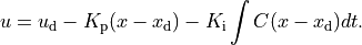
The number of outputs that are to be integrated
must match the number of additional columns in the K matrix. If an
estimator is specified, will be used in place of
.
As an example, consider the servo-mechanism model servomech
described in creating nonlinear models.
We construct a state space controller by linearizing the system around
an equilibrium point, augmenting the model with an integrator, and
computing a state feedback that optimizes a quadratic cost function:
# System dynamics (with full state output)
servomech = ct.nlsys(
    servomech_update, None, name='servomech',
    params=servomech_params, states=['theta', 'thdot'],
    outputs=['theta', 'thdot'], inputs=['tau'])

# Find operating point with output angle pi/4
xeq, ueq = ct.find_operating_point(
    servomech, [0, 0], 0, y0=[np.pi/4, 0], iy=0)

# Compute linearization and augment with an integrator on angle
A, B, _, _ = ct.ssdata(servomech.linearize(xeq, ueq))
C = np.array([[1, 0]])  # theta
A_aug = np.block([
    [A, np.zeros((2, 1))],
    [C, np.zeros((1, 1))]
])
B_aug = np.block([[B], [0]])

# Compute LQR controller
K, _, _ = ct.lqr(A_aug, B_aug, np.diag([1, 1, 0.1]), 1)

# Create controller with integral action
ctrl, _ = ct.create_statefbk_iosystem(
    servomech, K, integral_action=C, name='ctrl')
The resulting controller now has internal dynamics corresponding to the integral action:
>>> print(ctrl)
<StateSpace>: ctrl
Inputs (5): ['xd[0]', 'xd[1]', 'ud[0]', 'theta', 'thdot']
Outputs (1): ['tau']
States (1): ['x[0]']

A = [[0.]]

B = [[-1.  0.  0.  1.  0.]]

C = [[-0.31622777]]

D = [[  3.76244547  19.21453568   1.          -3.76244547 -19.21453568]]
Adding gain scheduling
Finally, for the trajectory generation design pattern, gain scheduling
on the desired state , desired input
, or current state can be implemented by
setting the gain to a 2-tuple consisting of a list of gains and a list
of points at which the gains were computed, as well as a description
of the scheduling variables:
ctrl, clsys = ct.create_statefbk_iosystem(
    sys, ([g1, ..., gN], [p1, ..., pN]), gainsched_indices=[s1, ..., sq])
The list of indices can either be integers indicating the offset into
the controller input vector  or a
list of strings matching the names of the input signals. The
controller implemented in this case has the form
or a
list of strings matching the names of the input signals. The
controller implemented in this case has the form
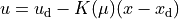
where  represents the scheduling variables. See gain
scheduled control for vehicle steering for an
example implementation of a gain scheduled controller (in the
alternative formulation section at the bottom of the file).
represents the scheduling variables. See gain
scheduled control for vehicle steering for an
example implementation of a gain scheduled controller (in the
alternative formulation section at the bottom of the file).
As an example, consider the following simple model of a mobile robot (“unicycle” model), which has dynamics given by

where , is the position of the robot in the plane,
 is the angle with respect to the axis,
 is the commanded velocity, and
  is the
commanded angular rate.
is the
commanded angular rate.
We define the nonlinear dynamics as follows:
def unicycle_update(t, x, u, params):
    return np.array([u[0] * np.cos(x[2]), u[0] * np.sin(x[2]), u[1]])

unicycle = ct.nlsys(
    unicycle_update, None, name='unicycle', states=3,
    inputs=['v', 'omega'], outputs=['x', 'y', 'theta'])
We construct a gain-scheduled controller by linearizing the dynamics
about a range of different speeds and angles :
# Speeds and angles at which to compute the gains
speeds = [1, 5, 10]
angles = np.linspace(0, np.pi/2, 4)
points = list(itertools.product(speeds, angles))

# Gains for each speed (using LQR controller)
Q = np.identity(unicycle.nstates)
R = np.identity(unicycle.ninputs)
gains = [np.array(ct.lqr(unicycle.linearize(
    [0, 0, angle], [speed, 0]), Q, R)[0]) for speed, angle in points]

# Create gain scheduled controller
ctrl, clsys = ct.create_statefbk_iosystem(
    unicycle, (gains, points), gainsched_indices=['v_d', 'th_d'], name='ctrl',
    inputs=['x_d', 'y_d', 'th_d', 'v_d', 'omega_d', 'x', 'y', 'theta'])
The resulting controller has the following structure:
>>> print(ctrl)
<NonlinearIOSystem>: ctrl
Inputs (8): ['x_d', 'y_d', 'th_d', 'v_d', 'omega_d', 'x', 'y', 'theta']
Outputs (2): ['v', 'omega']
States (0): []

Update: <function create_statefbk_iosystem.<locals>._control_update at 0x...>
Output: <function create_statefbk_iosystem.<locals>._control_output at 0x...>
This is a static, nonlinear controller, with the gains scheduled based
on the values of  (index 3) and
 (index 2).
Integral action and state estimation can also be used with gain scheduled controllers.