2. Python Control Systems Library (python-control) Tutorial

This Jupyter notebook contains an introduction to the basic operations in the Python Control Systems Library (python-control), a Python package for control system design. The tutorial consists of two examples:

Example 1: Open loop analysis of a coupled mass spring system
Example 2: Trajectory tracking for a kinematic car model

2.1. Initialization

The python-control package can be installed using pip or from conda-forge. The code below will import the control toolbox either from your local installation or via pip. We use the prefix ct to access control toolbox commands:

[1]:

# Import the packages needed for the examples included in this notebook
import numpy as np
import matplotlib.pyplot as plt

# Import the python-control package
try:
    import control as ct
    print("python-control", ct.__version__)
except ImportError:
    %pip install control
    import control as ct

python-control 0.10.1.dev324+g2fd3802a.d20241218

Installation notes

If you get an error importing the control package, it may be that it is not in your current Python path. You can fix this by setting the PYTHONPATH environment variable to include the directory where the python-control package is located. If you are invoking Jupyter from the command line, try using a command of the form

PYTHONPATH=/path/to/python-control jupyter notebook

If you are using Google Colab, use the following command at the top of the notebook to install the control package:

%pip install control

(The import code above automatically runs this command if needed.)

For the examples below, you will need version 0.10.0 or higher of the python-control toolbox. You can find the version number using the command

print(ct.__version__)

More information on Python, NumPy, python-control

2.2. Example 1: Open loop analysis of a coupled mass spring system

Consider the spring mass system below:

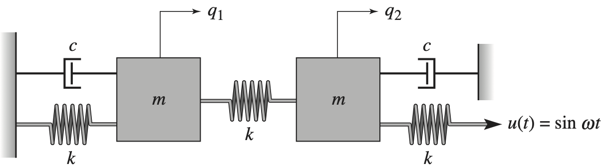
2768ca3692964e5eaf247f3dc8d1b9b4

We wish to analyze the time and frequency response of this system using a variety of python-control functions for linear systems analysis.

System dynamics

The dynamics of the system can be written as

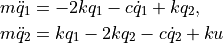
$\begin{aligned} m \ddot{q}_1 &= -2 k q_1 - c \dot{q}_1 + k q_2, \\ m \ddot{q}_2 &= k q_1 - 2 k q_2 - c \dot{q}_2 + ku \end{aligned}$

or in state space form:

$\begin{aligned} \dfrac{dx}{dt} &= \begin{bmatrix} 0 & 0 & 1 & 0 \\ 0 & 0 & 0 & 1 \\[0.5ex] -\dfrac{2k}{m} & \dfrac{k}{m} & -\dfrac{c}{m} & 0 \\[0.5ex] \dfrac{k}{m} & -\dfrac{2k}{m} & 0 & -\dfrac{c}{m} \end{bmatrix} x + \begin{bmatrix} 0 \\ 0 \\[0.5ex] 0 \\[1ex] \dfrac{k}{m} \end{bmatrix} u. \end{aligned}$

[2]:

# Define the parameters for the system
m, c, k = 1, 0.1, 2
# Create a linear system
A = np.array([
    [0, 0, 1, 0],
    [0, 0, 0, 1],
    [-2*k/m, k/m, -c/m, 0],
    [k/m, -2*k/m, 0, -c/m]
])
B = np.array([[0], [0], [0], [k/m]])
C = np.array([[1, 0, 0, 0], [0, 1, 0, 0]])
D = 0

sys = ct.ss(A, B, C, D, outputs=['q1', 'q2'], name="coupled spring mass")
print(sys)

<StateSpace>: coupled spring mass
Inputs (1): ['u[0]']
Outputs (2): ['q1', 'q2']
States (4): ['x[0]', 'x[1]', 'x[2]', 'x[3]']

A = [[ 0.   0.   1.   0. ]
     [ 0.   0.   0.   1. ]
     [-4.   2.  -0.1  0. ]
     [ 2.  -4.   0.  -0.1]]

B = [[0.]
     [0.]
     [0.]
     [2.]]

C = [[1. 0. 0. 0.]
     [0. 1. 0. 0.]]

D = [[0.]
     [0.]]

Initial response

The initial_response function can be used to compute the response of the system with no input, but starting from a given initial condition. This function returns a response object, which can be used for plotting.

[3]:

response = ct.initial_response(sys, X0=[1, 0, 0, 0])
cplt = response.plot()

../_images/examples_python-control_tutorial_8_0.png

If you want to play around with the way the data are plotted, you can also use the response object to get direct access to the states and outputs.

[4]:

# Plot the outputs of the system on the same graph, in different colors
t = response.time
x = response.states
plt.plot(t, x[0], 'b', t, x[1], 'r')
plt.legend(['$x_1$', '$x_2$'])
plt.xlim(0, 50)
plt.ylabel('States')
plt.xlabel('Time [s]')
plt.title("Initial response from $x_1 = 1$, $x_2 = 0$");

../_images/examples_python-control_tutorial_10_0.png

There are also lots of options available in initial_response and .plot() for tuning the plots that you get.

[5]:

for X0 in [[1, 0, 0, 0], [0, 2, 0, 0], [1, 2, 0, 0], [0, 0, 1, 0], [0, 0, 2, 0]]:
  response = ct.initial_response(sys, T=20, X0=X0)
  response.plot(label=f"{X0=}")

../_images/examples_python-control_tutorial_12_0.png

Step response

Similar to initial_response, you can also generate a step response for a linear system using the step_response function, which returns a time response object:

[6]:

cplt = ct.step_response(sys).plot()

../_images/examples_python-control_tutorial_14_0.png

We can analyze the properties of the step response using the stepinfo command:

[7]:

step_info = ct.step_info(sys)
print("Input 0, output 0 rise time = ",
      step_info[0][0]['RiseTime'], "seconds\n")
step_info

Input 0, output 0 rise time =  0.6153902252990775 seconds

[7]:

[[{'RiseTime': 0.6153902252990775,
   'SettlingTime': 89.02645259326653,
   'SettlingMin': -0.13272845655369417,
   'SettlingMax': 0.9005994876222034,
   'Overshoot': 170.17984628666102,
   'Undershoot': 39.81853696610825,
   'Peak': 0.9005994876222034,
   'PeakTime': 2.3589958636464634,
   'SteadyStateValue': 0.33333333333333337}],
 [{'RiseTime': 0.6153902252990775,
   'SettlingTime': 73.6416969607896,
   'SettlingMin': 0.2276019820782241,
   'SettlingMax': 1.13389337710215,
   'Overshoot': 70.08400656532254,
   'Undershoot': 0.0,
   'Peak': 1.13389337710215,
   'PeakTime': 6.564162403190159,
   'SteadyStateValue': 0.6666666666666665}]]

Note that by default the inputs are not included in the step response plot (since they are a bit boring), but you can change that:

[8]:

stepresp = ct.step_response(sys)
cplt = stepresp.plot(plot_inputs=True)

../_images/examples_python-control_tutorial_18_0.png

[9]:

# Plot the inputs on top of the outputs
cplt = stepresp.plot(plot_inputs='overlay')

../_images/examples_python-control_tutorial_19_0.png

[10]:

# Look at the "shape" of the step response
print(f"{stepresp.time.shape=}")
print(f"{stepresp.inputs.shape=}")
print(f"{stepresp.states.shape=}")
print(f"{stepresp.outputs.shape=}")

stepresp.time.shape=(1348,)
stepresp.inputs.shape=(1, 1, 1348)
stepresp.states.shape=(4, 1, 1348)
stepresp.outputs.shape=(2, 1, 1348)

Forced response

To compute the response to an input, using the convolution equation, we can use the forced_response function:

[11]:

T = np.linspace(0, 50, 500)
U1 = np.cos(T)
U2 = np.sin(3 * T)

resp1 = ct.forced_response(sys, T, U1)
resp2 = ct.forced_response(sys, T, U2)
resp3 = ct.forced_response(sys, T, U1 + U2)

# Plot the individual responses
resp1.sysname = 'U1'; resp1.plot(color='b')
resp2.sysname = 'U2'; resp2.plot(color='g')
resp3.sysname = 'U1 + U2'; resp3.plot(color='r');

../_images/examples_python-control_tutorial_22_0.png

[12]:

# Show that the system response is linear
cplt = resp3.plot(label="G(U1 + U2)")
cplt.axes[0, 0].plot(resp1.time, resp1.outputs[0] + resp2.outputs[0], 'k--', label="G(U1) + G(U2)")
cplt.axes[1, 0].plot(resp1.time, resp1.outputs[1] + resp2.outputs[1], 'k--')
cplt.axes[2, 0].plot(resp1.time, resp1.inputs[0] + resp2.inputs[0], 'k--')
cplt.axes[0, 0].legend(loc='upper right', fontsize='x-small');

../_images/examples_python-control_tutorial_23_0.png

[13]:

# Show that the forced response from non-zero initial condition is not linear
X0 = [1, 0, 0, 0]
resp1 = ct.forced_response(sys, T, U1, X0=X0)
resp2 = ct.forced_response(sys, T, U2, X0=X0)
resp3 = ct.forced_response(sys, T, U1 + U2, X0=X0)

cplt = resp3.plot(label="G(U1 + U2)")
cplt.axes[0, 0].plot(resp1.time, resp1.outputs[0] + resp2.outputs[0], 'k--', label="G(U1) + G(U2)")
cplt.axes[1, 0].plot(resp1.time, resp1.outputs[1] + resp2.outputs[1], 'k--')
cplt.axes[2, 0].plot(resp1.time, resp1.inputs[0] + resp2.inputs[0], 'k--')
cplt.axes[0, 0].legend(loc='upper right', fontsize='x-small');

../_images/examples_python-control_tutorial_24_0.png

Frequency response

[14]:

# Manual computation of the frequency response
resp = ct.input_output_response(sys, T, np.sin(1.35 * T))

cplt = resp.plot(
    plot_inputs='overlay',
    legend_map=np.array([['lower left'], ['lower left']]),
    label=[['q1', 'u[0]'], ['q2', None]])

../_images/examples_python-control_tutorial_26_0.png

The magnitude and phase of the frequency response is controlled by the transfer function,

$G(s) = C (sI - A)^{-1} B + D$

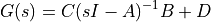
which can be computed using the ss2tf function:

[15]:

try:
    G = ct.ss2tf(sys, name='u to q1, q2')
except ct.ControlMIMONotImplemented:
    # Create SISO transfer functions, in case we don't have slycot
    G = ct.ss2tf(sys[0, 0], name='u to q1')
print(G)

<TransferFunction>: u to q1, q2
Inputs (1): ['u[0]']
Outputs (2): ['q1', 'q2']

Input 1 to output 1:

                    4
  -------------------------------------
  s^4 + 0.2 s^3 + 8.01 s^2 + 0.8 s + 12

Input 1 to output 2:

            2 s^2 + 0.2 s + 8
  -------------------------------------
  s^4 + 0.2 s^3 + 8.01 s^2 + 0.8 s + 12

[16]:

# Gain and phase for the simulation above
from math import pi
val = G(1.35j)
print(f"{G(1.35j)=}")
print(f"Gain: {np.absolute(val)}")
print(f"Phase: {np.angle(val)}", " (", np.angle(val) * 180/pi, "deg)")

G(1.35j)=array([[3.33005647-2.70686327j],
       [3.80831226-2.72231858j]])
Gain: [[4.29143157]
 [4.681267  ]]
Phase: [[-0.6825322 ]
 [-0.62061375]]  ( [[-39.10621449]
 [-35.55854848]] deg)

[17]:

# Gain and phase at s = 0 (= steady state step response)
print(f"{G(0)=}")
print("Final value of step response:", stepresp.outputs[0, 0, -1])

G(0)=array([[0.33333333+0.j],
       [0.66666667+0.j]])
Final value of step response: 0.33297541813724874

The frequency response across all frequencies can be computed using the frequency_response function:

[18]:

freqresp = ct.frequency_response(sys)
cplt = freqresp.plot()

../_images/examples_python-control_tutorial_32_0.png

By default, frequency responses are plotted using a “Bode plot”, which plots the log of the magnitude and the (linear) phase against the log of the forcing frequency.

You can also call the Bode plot command directly, and change the way the data are presented:

[19]:

cplt = ct.bode_plot(sys, overlay_outputs=True)

../_images/examples_python-control_tutorial_34_0.png

Note the “dip” in the frequency response for $q_2$ at frequency 2 rad/sec, which corresponds to a “zero” of the transfer function.

2.3. Example 2: Trajectory tracking for a kinematic vehicle model

This example illustrates the use of python-control to model, analyze, and design nonlinear control systems.

We make use of a simple model for a vehicle navigating in the plane, known as the “bicycle model”. The kinematics of this vehicle can be written in terms of the contact point $(x, y)$ and the angle $\theta$ of the vehicle with respect to the horizontal axis:

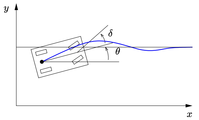
c4baf58b824f423aa34cfc29aff582cb

$\large\begin{aligned} \dot x &= \cos\theta\, v \\ \dot y &= \sin\theta\, v \\ \dot\theta &= \frac{v}{l} \tan \delta \end{aligned}$

The input $v$ represents the velocity of the vehicle and the input $\delta$ represents the turning rate. The parameter $l$ is the wheelbase.

System Definiton

We define the dynamics of the system that we are going to use for the control design. The dynamics of the system will be of the form

$\dot x = f(x, u), \qquad y = h(x, u)$

where $x$ is the state vector for the system, $u$ represents the vector of inputs, and $y$ represents the vector of outputs.

The python-control package allows definition of input/output systems using the InputOutputSystem class and its various subclasess, including the NonlinearIOSystem class that we use here. A NonlinearIOSystem object is created by defining the update law ( $f(x, u)$ ) and the output map ( $h(x, u)$ ), and then calling the factory function ct.nlsys.

For the example in this notebook, we will be controlling the steering of a vehicle, using a “bicycle” model for the dynamics of the vehicle. A more complete description of the dynamics of this system are available in Example 3.11 of Feedback Systems by Astrom and Murray (2020).

[20]:

# Define the update rule for the system, f(x, u)
# States: x, y, theta (postion and angle of the center of mass)
# Inputs: v (forward velocity), delta (steering angle)
def vehicle_update(t, x, u, params):
    # Get the parameters for the model
    a = params.get('refoffset', 1.5)        # offset to vehicle reference point
    b = params.get('wheelbase', 3.)         # vehicle wheelbase
    maxsteer = params.get('maxsteer', 0.5)  # max steering angle (rad)

    # Saturate the steering input
    delta = np.clip(u[1], -maxsteer, maxsteer)
    alpha = np.arctan2(a * np.tan(delta), b)

    # Return the derivative of the state
    return np.array([
        u[0] * np.cos(x[2] + alpha),    # xdot = cos(theta + alpha) v
        u[0] * np.sin(x[2] + alpha),    # ydot = sin(theta + alpha) v
        (u[0] / a) * np.sin(alpha)      # thdot = v sin(alpha) / a
    ])

# Define the readout map for the system, h(x, u)
# Outputs: x, y (planar position of the center of mass)
def vehicle_output(t, x, u, params):
    return x

# Default vehicle parameters (including nominal velocity)
vehicle_params={'refoffset': 1.5, 'wheelbase': 3, 'velocity': 15,
                'maxsteer': 0.5}

# Define the vehicle steering dynamics as an input/output system
vehicle = ct.nlsys(
    vehicle_update, vehicle_output, states=3, name='vehicle',
    inputs=['v', 'delta'], outputs=['x', 'y', 'theta'], params=vehicle_params)

Open loop simulation

After these operations, the vehicle object references the nonlinear model for the system. This system can be simulated to compute a trajectory for the system. Here we command a velocity of 10 m/s and turn the wheel back and forth at one Hertz.

[21]:

# Define the time interval that we want to use for the simualation
timepts = np.linspace(0, 10, 1000)

# Define the inputs
U = [
    10 * np.ones_like(timepts),          # velocity
    0.1 * np.sin(timepts * 2*np.pi)      # steering angle
]

# Simulate the system dynamics, starting from the origin
response = ct.input_output_response(vehicle, timepts, U, 0)
time, outputs, inputs = response.time, response.outputs, response.inputs

We can plot the results using standard matplotlib commands:

[22]:

# Create a figure to plot the results
fig, ax = plt.subplots(2, 1)

# Plot the results in the xy plane
ax[0].plot(outputs[0], outputs[1])
ax[0].set_xlabel("$x$ [m]")
ax[0].set_ylabel("$y$ [m]")

# Plot the inputs
ax[1].plot(timepts, U[0])
ax[1].set_ylim(0, 12)
ax[1].set_xlabel("Time $t$ [s]")
ax[1].set_ylabel("Velocity $v$ [m/s]")
ax[1].yaxis.label.set_color('blue')

rightax = ax[1].twinx()       # Create an axis in the right
rightax.plot(timepts, U[1], color='red')
rightax.set_ylim(None, 0.5)
rightax.set_ylabel(r"Steering angle $\phi$ [rad]")
rightax.yaxis.label.set_color('red')

fig.tight_layout()

../_images/examples_python-control_tutorial_42_0.png

Notice that there is a small drift in the $y$ position despite the fact that the steering wheel is moved back and forth symmetrically around zero. Exercise: explain what might be happening.

Linearize the system around a trajectory

We choose a straight path along the $x$ axis at a speed of 10 m/s as our desired trajectory and then linearize the dynamics around the initial point in that trajectory.

[23]:

# Create the desired trajectory
Ud = np.array([10 * np.ones_like(timepts), np.zeros_like(timepts)])
Xd = np.array([10 * timepts, 0 * timepts, np.zeros_like(timepts)])

# Now linizearize the system around this trajectory
linsys = vehicle.linearize(Xd[:, 0], Ud[:, 0])

[24]:

# Check on the eigenvalues of the open loop system
np.linalg.eigvals(linsys.A)

[24]:

array([0., 0., 0.])

We see that all eigenvalues are zero, corresponding to a single integrator in the $x$ (longitudinal) direction and a double integrator in the $y$ (lateral) direction.

Compute a state space (LQR) control law

We can now compute a feedback controller around the trajectory. We choose a simple LQR controller here, but any method can be used.

[25]:

# Compute LQR controller
K, S, E = ct.lqr(linsys, np.diag([1, 1, 1]), np.diag([1, 1]))

[26]:

# Check on the eigenvalues of the closed loop system
np.linalg.eigvals(linsys.A - linsys.B @ K)

[26]:

array([-1.        +0.j        , -5.06896878+2.76385399j,
       -5.06896878-2.76385399j])

The closed loop eigenvalues have negative real part, so the closed loop (linear) system will be stable about the operating trajectory.

Create a controller with feedforward and feedback

We now create an I/O system representing the control law. The controller takes as an input the desired state space trajectory $x_\text{d}$ and the nominal input $u_\text{d}$ . It outputs the control law

$u = u_\text{d} - K(x - x_\text{d}).$

[27]:

# Define the output rule for the controller
# States: none (=> no update rule required)
# Inputs: z = [xd, ud, x]
# Outputs: v (forward velocity), delta (steering angle)
def control_output(t, x, z, params):
    # Get the parameters for the model
    K = params.get('K', np.zeros((2, 3)))   # nominal gain

    # Split up the input to the controller into the desired state and nominal input
    xd_vec = z[0:3]    # desired state ('xd', 'yd', 'thetad')
    ud_vec = z[3:5]    # nominal input ('vd', 'deltad')
    x_vec = z[5:8]     # current state ('x', 'y', 'theta')

    # Compute the control law
    return ud_vec - K @ (x_vec - xd_vec)

# Define the controller system
control = ct.nlsys(
    None, control_output, name='control',
    inputs=['xd', 'yd', 'thetad', 'vd', 'deltad', 'x', 'y', 'theta'],
    outputs=['v', 'delta'], params={'K': K})

Because we have named the signals in both the vehicle model and the controller in a compatible way, we can use the autoconnect feature of the interconnect() function to create the closed loop system.

[28]:

# Build the closed loop system
vehicle_closed = ct.interconnect(
    (vehicle, control),
    inputs=['xd', 'yd', 'thetad', 'vd', 'deltad'],
    outputs=['x', 'y', 'theta']
)

Closed loop simulation

We now command the system to follow a trajectory and use the linear controller to correct for any errors.

The desired trajectory is a given by a longitudinal position that tracks a velocity of 10 m/s for the first 5 seconds and then increases to 12 m/s and a lateral position that varies sinusoidally by $\pm 0.5$ m around the centerline. The nominal inputs are not modified, so that feedback is required to obtained proper trajectory tracking.

[29]:

Xd = np.array([
    10 * timepts + 2 * (timepts-5) * (timepts > 5),
    0.5 * np.sin(timepts * 2*np.pi),
    np.zeros_like(timepts)
])

Ud = np.array([10 * np.ones_like(timepts), np.zeros_like(timepts)])

# Simulate the system dynamics, starting from the origin
resp = ct.input_output_response(
    vehicle_closed, timepts, np.vstack((Xd, Ud)), 0)
time, outputs = resp.time, resp.outputs

[30]:

# Plot the results in the xy plane
plt.plot(Xd[0], Xd[1], 'b--')      # desired trajectory
plt.plot(outputs[0], outputs[1])   # actual trajectory
plt.xlabel("$x$ [m]")
plt.ylabel("$y$ [m]")
plt.ylim(-1, 2)

# Add a legend
plt.legend(['desired', 'actual'], loc='upper left')

# Compute and plot the velocity
rightax = plt.twinx()       # Create an axis in the right
rightax.plot(Xd[0, :-1], np.diff(Xd[0]) / np.diff(timepts), 'r--')
rightax.plot(outputs[0, :-1], np.diff(outputs[0]) / np.diff(timepts), 'r-')
rightax.set_ylim(0, 13)
rightax.set_ylabel("$x$ velocity [m/s]")
rightax.yaxis.label.set_color('red')

../_images/examples_python-control_tutorial_58_0.png

We see that there is a small error in each axis. By adjusting the weights in the LQR controller we can adjust the steady state error (try it!)

2.4. Computing environment

[31]:

print("Control version:", ct.__version__)
if ct.slycot_check():
    import slycot
    print("Slycot version:", slycot.__version__)
else:
    print("Slycot version: not installed")
print("NumPy version:", np.__version__)

Control version: 0.10.1.dev324+g2fd3802a.d20241218
Slycot version: 0.6.0
NumPy version: 2.2.0