Simulating interconnections of systems

Sawyer B. Fuller 2023.03

This example creates a precise simulation of a sampled-data control system consisting of discrete-time controller(s) and continuous-time plant dynamics like the following.

In many cases, it is sufficient to use a discretized model of your plant using a zero-order-hold for control design because it is exact at the sampling instants. However, a more complete simulation of your sampled-data feedback control system may be desired if you want to additionally

• observe behavior that occurs between sampling instants,

• model the effect of time delays,

• simulate your controller operating with a nonlinear plant, which may not have an exact zero-order-hold discretization

Here, we include helper functions that can be used in conjunction with the Python Control Systems Library to create a simulation of such a closed-loop system, providing a Simulink-like interconnection system.

Our approach is to discretize all of the constituent systems, including the plant and controller(s) with a much shorter time step simulation_dt that we specify. With this, behavior that occurs between the sampling instants of our discrete-time controller can be observed.

import numpy as np # arrays
import matplotlib.pyplot as plt # plots
%config InlineBackend.figure_format='retina' # high-res plots

import control as ct # control systems library

We will assume the controller is a discrete-time system of the form

For this course we will primarily work with linear systems of the form

The plant is assumed to be continuous-time, of the form

,

For this course, we will design our controller using a linearized model of the plant given by

,

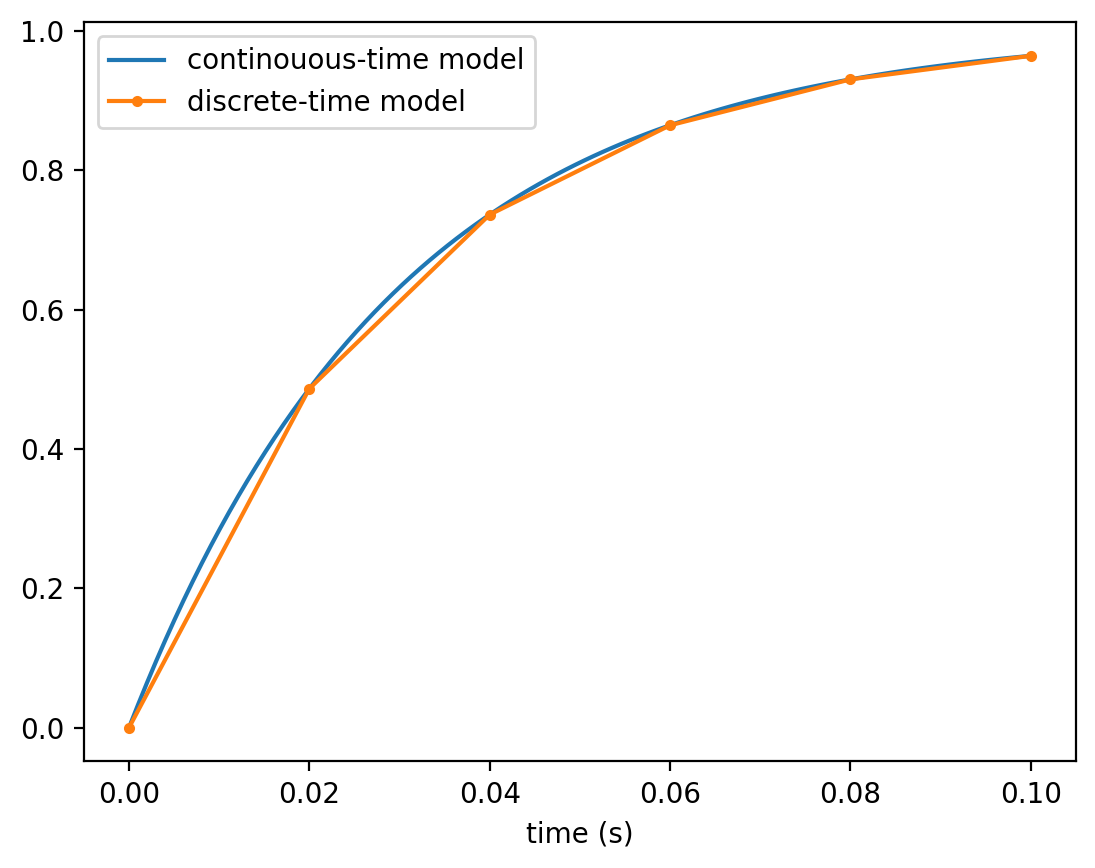
The first step to create our interconnected system is to create a discrete-time model of the plant, which uses the short time interval simulation_dt. Each subsystem gets signal names according to the diagram above, and we use interconnect to automatically connect signals of the same name.

# continuous-time plant model
plantcont = ct.tf(1, (0.03, 1), inputs='u', outputs='y')
t, y = ct.step_response(plantcont, 0.1)
plt.plot(t, y, label='continouous-time model')

# create discrete-time simulation form assuming a zero-order hold
simulation_dt = 0.02 # time step for numerical simulation ("numerical integration")
plant_simulator = ct.c2d(plantcont, simulation_dt, 'zoh')

t, y = ct.step_response(plant_simulator, 0.1)
plt.plot(t, y, '.-', label='discrete-time model')
plt.legend()
plt.xlabel('time (s)');

Next we create a model of a sampled-data controller that operates as a nonlinear discrete-time system with a much shorter time step than the controller’s sampling time Ts.

def sampled_data_controller(controller, plant_dt):
    """
    Create a (discrete-time, non-linear) system that models the behavior
    of a digital controller.

    The system that is returned models the behavior of a sampled-data
    controller, consisting of a sampler and a digital-to-analog converter.
    The returned system is discrete-time, and its timebase `plant_dt` is
    much smaller than the sampling interval of the controller,
    `controller.dt`, to insure that continuous-time dynamics of the plant
    are accurately simulated. This system must be interconnected
    to a plant with the same dt. The controller's sampling period must be
    greater than or equal to `plant_dt`, and an integral multiple of it.
    The plant that is connected to it must be converted to a discrete-time
    approximation with a sampling interval that is also `plant_dt`. A
    controller that is a pure gain must have its `dt` specified (not None).
    """
    assert ct.isdtime(controller, True), "controller must be discrete-time"
    controller = ct.ss(controller) # convert to state-space if not already
    # the following is used to ensure the number before '%' is a bit larger
    one_plus_eps = 1 + np.finfo(float).eps
    assert np.isclose(0, controller.dt*one_plus_eps % plant_dt), \
        "plant_dt must be an integral multiple of the controller's dt"
    nsteps = int(round(controller.dt / plant_dt))
    step = 0
    def updatefunction(t, x, u, params): # update if it is time to sample
        nonlocal step
        if step == 0:
            x = controller._rhs(t, x, u)
        step += 1
        if step == nsteps:
            step = 0
        return x
    y = np.zeros((controller.noutputs, 1))
    def outputfunction(t, x, u, params): # update if it is time to sample
        nonlocal y
        if step == 0: # last time updatefunction was called was a sample time
            y = controller._out(t, x, u)
        return y
    return ct.ss(updatefunction, outputfunction, dt=plant_dt,
                 name=controller.name, inputs=controller.input_labels,
                 outputs=controller.output_labels, states=controller.state_labels)

# create discrete-time controller with some dynamics
controller_Ts = .1 # sampling interval of controller
controller = ct.tf(1, [1, -.9], controller_Ts, inputs='e', outputs='u')

# create model of controller with a much shorter sampling time for simulation
controller_simulator = sampled_data_controller(controller, simulation_dt)

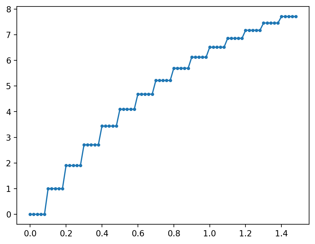
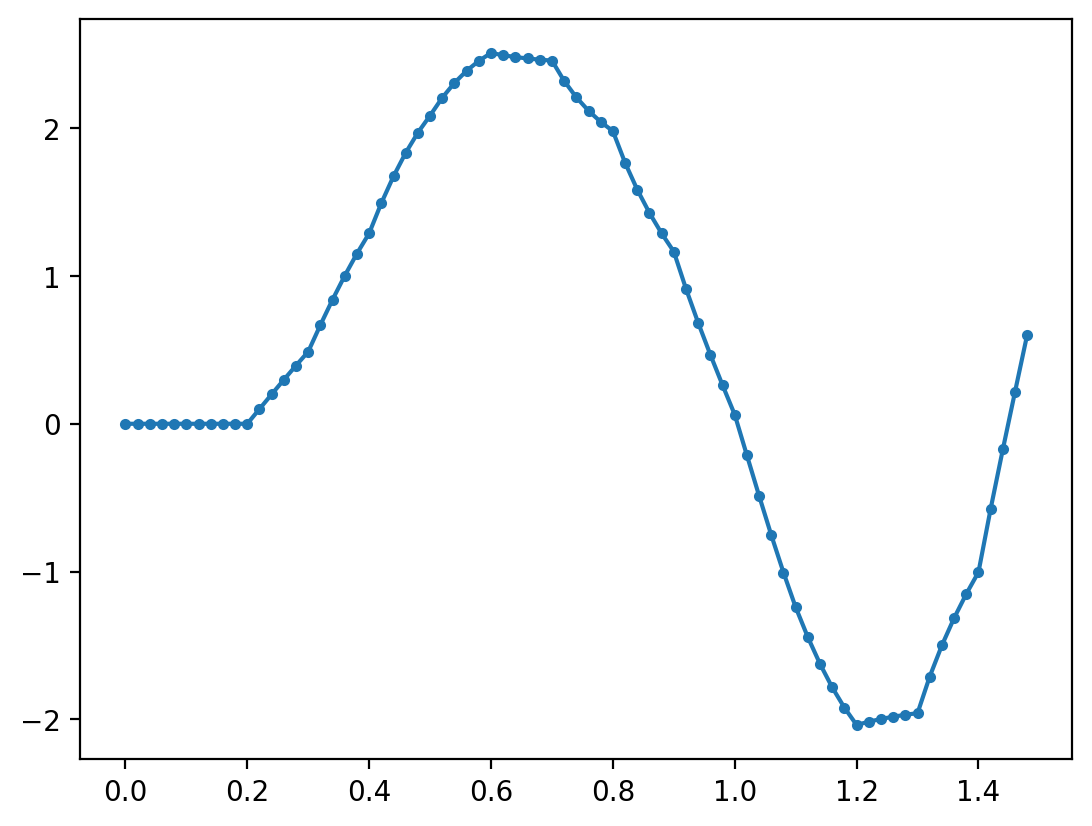
If the model is simulated with a short time step, its staircase output behavior can be observed. Because the controller model is nonlinear, we must use ct.input_output_response.

time = np.arange(0, 1.5, simulation_dt)
step_input = np.ones_like(time)
t, y = ct.input_output_response(controller_simulator, time, step_input)
plt.plot(t, y, '.-');

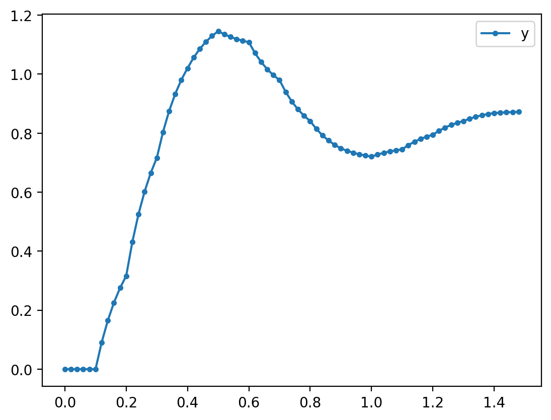
simulating a closed-loop system

Now we are able to construct a closed-loop simulation of the full sampled-data system.

plantcont = ct.tf(.5, (0.1, 1), inputs='u', outputs='y')
u_summer  = ct.summing_junction(inputs=['-y', 'r'], outputs='e')

plant_simulator = ct.c2d(plantcont, simulation_dt, 'zoh')
# system from r to y
Gyr_simulator = ct.interconnect([controller_simulator, plant_simulator, u_summer],
    inputs='r', outputs=['y', 'u'])

# simulate
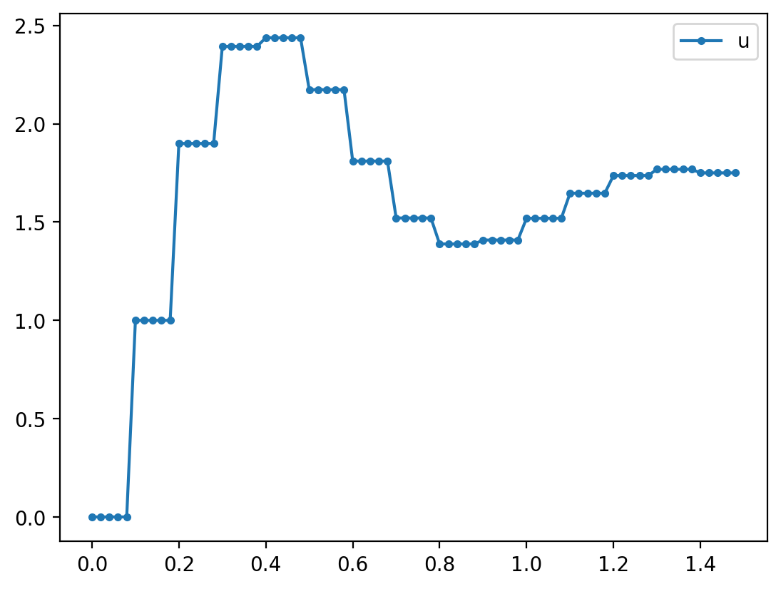
t, y = ct.input_output_response(Gyr_simulator, time, step_input)
y, u = y # extract respones
plt.plot(t, y, '.-', label='y')
plt.legend()
plt.figure()
plt.plot(t, u, '.-', label='u')
plt.legend();

time delays

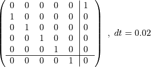
Given that all of the interconnected systems are being simulated in discrete-time with the same small time interval simulation_dt, we can construct a system that implements time delays by suitable choice of $A, B, C, $ and matrices. For example, a 3-step delay has the form

The following function creates an arbitrarily-long time delay system, up to the nearest .

def time_delay_system(delay, dt, inputs=1, outputs=1, **kwargs):
    """
    creates a pure time delay discrete-time system.
    time delay is equal to nearest whole number of `dt`s."""
    assert delay >= 0, "delay must be greater than or equal to zero"
    n = int(round(delay/dt))
    ninputs = inputs if isinstance(inputs, (int, float)) else len(inputs)
    assert ninputs == 1, "only one input supported"
    A = np.eye(n, k=-1)
    B = np.eye(n, 1)
    C = np.eye(1, n, k=n-1)
    D = np.zeros((1,1))
    return ct.ss(A, B, C, D, dt, inputs=inputs, outputs=outputs, **kwargs)

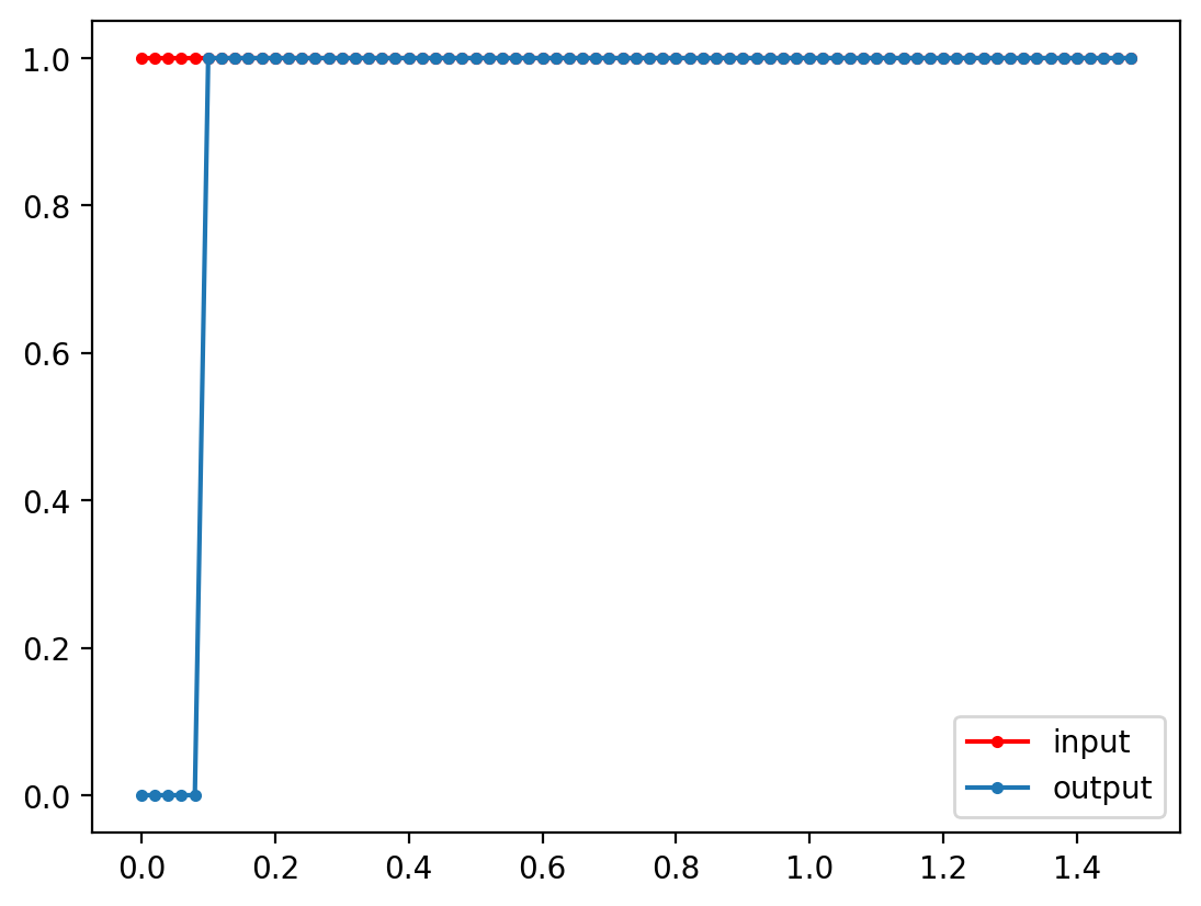
The step response of the time-delay system is shifted to the right.

delayer = time_delay_system(.1, simulation_dt, inputs='u', outputs='ud')
t, y  = ct.input_output_response(delayer, time, step_input)
plt.plot(time, step_input, 'r.-', label='input')
plt.plot(t, y, '.-', label='output')
plt.legend()
delayer

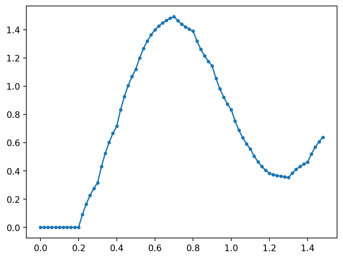
We can incorporate this delay into our closed-loop system. The time delay shifts the response to the right and brings the system closer to instability.

# incorporate delay into system by relabeling plant input signal
plant_simulator = ct.ss(plant_simulator, inputs='ud', outputs='y')

# system from r to y
Gyr_simulator = ct.interconnect([controller_simulator, plant_simulator, u_summer, delayer],
                                inputs='r', outputs='y')

# simulate
t, y = ct.input_output_response(Gyr_simulator, time, step_input)
plt.plot(t, y, '.-');

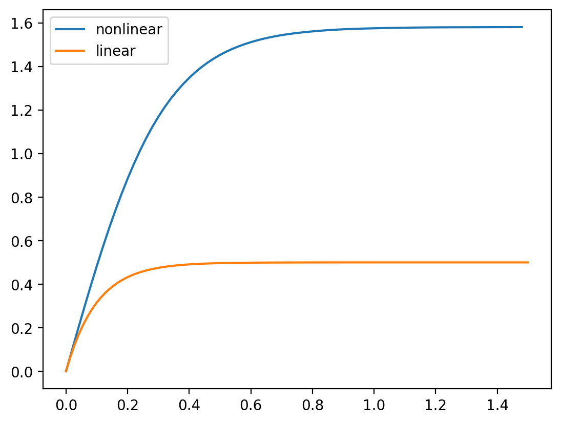
We can also observe how the dynamics behave with a nonlinear plant.

def nonlinear_plant_dynamics(t, x, u, params):
    return -10 * x * abs(x) +  u
def nonlinear_plant_output(t, x, u, params):
    return 5 * x
nonlinear_plant = ct.ss(nonlinear_plant_dynamics, nonlinear_plant_output,
                        inputs='ud', outputs='y', states=1)

# compare step responses
t, y = ct.input_output_response(nonlinear_plant, time, step_input)
plt.plot(t, y, label='nonlinear')
t, y = ct.step_response(plantcont, 1.5)
plt.plot(t, y, label='linear')
plt.legend();

now create a closed-loop system.

Note that this system is not intended to show operation of well-designed feedback control system.

# create zero-order hold approximation of plant2 dynamics
def discrete_nonlinear_plant_dynamics(t, x, u, params):
    return x + simulation_dt * nonlinear_plant_dynamics(t, x, u, params)
nonlinear_plant_simulator = ct.ss(discrete_nonlinear_plant_dynamics, nonlinear_plant_output,
                                  dt=simulation_dt,
                                  inputs='ud', outputs='y', states=1)

# system from r to y
nonlinear_Gyr_simulator = ct.interconnect([controller_simulator, nonlinear_plant_simulator, u_summer, delayer],
                                inputs='r', outputs=['y', 'u'])

# simulate
t, y = ct.input_output_response(nonlinear_Gyr_simulator, time, step_input)
plt.plot(t, y[0],'.-');