Moving Horizon Estimation
Richard M. Murray, 24 Feb 2023
In this notebook we illustrate the implementation of moving horizon estimation (MHE)
[1]:
import numpy as np
import scipy as sp
import matplotlib.pyplot as plt
import control as ct

import control.optimal as opt
import control.flatsys as fs
System Description
The dynamics of the system with disturbances on the  and
and  variables is given by
The measured values of the system are the position and orientation, with added noise  ,
,  , and
, and  :
:
[2]:
# pvtol = nominal system (no disturbances or noise)
# noisy_pvtol = pvtol w/ process disturbances and sensor noise
from pvtol import pvtol, pvtol_noisy, plot_results
import pvtol as pvt

# Find the equiblirum point corresponding to the origin
xe, ue = ct.find_eqpt(
    pvtol, np.zeros(pvtol.nstates),
    np.zeros(pvtol.ninputs), [0, 0, 0, 0, 0, 0],
    iu=range(2, pvtol.ninputs), iy=[0, 1])

# Initial condition = 2 meters right, 1 meter up
x0, u0 = ct.find_eqpt(
    pvtol, np.zeros(pvtol.nstates),
    np.zeros(pvtol.ninputs), np.array([2, 1, 0, 0, 0, 0]),
    iu=range(2, pvtol.ninputs), iy=[0, 1])

# Extract the linearization for use in LQR design
pvtol_lin = pvtol.linearize(xe, ue)
A, B = pvtol_lin.A, pvtol_lin.B

print(pvtol, "\n")
print(pvtol_noisy)
<FlatSystem>: pvtol
Inputs (2): ['F1', 'F2']
Outputs (6): ['x0', 'x1', 'x2', 'x3', 'x4', 'x5']
States (6): ['x0', 'x1', 'x2', 'x3', 'x4', 'x5']

Update: <function _pvtol_update at 0x113697ac0>
Output: <function _pvtol_output at 0x113697a30>

Forward: <function _pvtol_flat_forward at 0x167b2fd00>
Reverse: <function _pvtol_flat_reverse at 0x167b2fbe0>

<NonlinearIOSystem>: pvtol_noisy
Inputs (7): ['F1', 'F2', 'Dx', 'Dy', 'Nx', 'Ny', 'Nth']
Outputs (6): ['x0', 'x1', 'x2', 'x3', 'x4', 'x5']
States (6): ['x0', 'x1', 'x2', 'x3', 'x4', 'x5']

Update: <function _noisy_update at 0x167b2fc70>
Output: <function _noisy_output at 0x167b2ff40>
Control Design
[3]:
#
# LQR design w/ physically motivated weighting
#
# Shoot for 10 cm error in x, 10 cm error in y.  Try to keep the angle
# less than 5 degrees in making the adjustments.  Penalize side forces
# due to loss in efficiency.
#

Qx = np.diag([100, 10, (180/np.pi) / 5, 0, 0, 0])
Qu = np.diag([10, 1])
K, _, _ = ct.lqr(A, B, Qx, Qu)

# Compute the full state feedback solution
lqr_ctrl, _ = ct.create_statefbk_iosystem(pvtol, K)

# Define the closed loop system that will be used to generate trajectories
lqr_clsys = ct.interconnect(
    [pvtol_noisy, lqr_ctrl],
    inplist = lqr_ctrl.input_labels[0:pvtol.ninputs + pvtol.nstates] + \
        pvtol_noisy.input_labels[pvtol.ninputs:],
    inputs = lqr_ctrl.input_labels[0:pvtol.ninputs + pvtol.nstates] + \
        pvtol_noisy.input_labels[pvtol.ninputs:],
    outlist = pvtol.output_labels + lqr_ctrl.output_labels,
    outputs = pvtol.output_labels + lqr_ctrl.output_labels
)
print(lqr_clsys)
<InterconnectedSystem>: sys[4]
Inputs (13): ['xd[0]', 'xd[1]', 'xd[2]', 'xd[3]', 'xd[4]', 'xd[5]', 'ud[0]', 'ud[1]', 'Dx', 'Dy', 'Nx', 'Ny', 'Nth']
Outputs (8): ['x0', 'x1', 'x2', 'x3', 'x4', 'x5', 'F1', 'F2']
States (6): ['pvtol_noisy_x0', 'pvtol_noisy_x1', 'pvtol_noisy_x2', 'pvtol_noisy_x3', 'pvtol_noisy_x4', 'pvtol_noisy_x5']

Update: <function InterconnectedSystem.__init__.<locals>.updfcn at 0x167b58dc0>
Output: <function InterconnectedSystem.__init__.<locals>.outfcn at 0x167b58e50>
/Users/murray/src/python-control/murrayrm/control/statefbk.py:783: UserWarning: cannot verify system output is system state
  warnings.warn("cannot verify system output is system state")
[4]:
# Disturbance and noise intensities
Qv = np.diag([1e-2, 1e-2])
Qw = np.array([[1e-4, 0, 1e-5], [0, 1e-4, 1e-5], [1e-5, 1e-5, 1e-4]])

# Initial state covariance
P0 = np.eye(pvtol.nstates)
[5]:
# Create the time vector for the simulation
Tf = 6
timepts = np.linspace(0, Tf, 20)
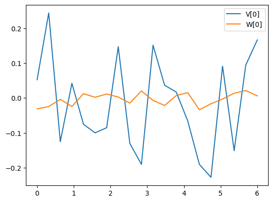
# Create representative process disturbance and sensor noise vectors
# np.random.seed(117) # avoid figures changing from run to run
V = ct.white_noise(timepts, Qv)
# V = np.clip(V0, -0.1, 0.1) # Hold for later
W = ct.white_noise(timepts, Qw)
# plt.plot(timepts, V0[0], 'b--', label="V[0]")
plt.plot(timepts, V[0], label="V[0]")
plt.plot(timepts, W[0], label="W[0]")
plt.legend();
[6]:
# Desired trajectory
xd, ud = xe, ue
# xd = np.vstack([
# np.sin(2 * np.pi * timepts / timepts[-1]),
# np.zeros((5, timepts.size))])
# ud = np.outer(ue, np.ones_like(timepts))
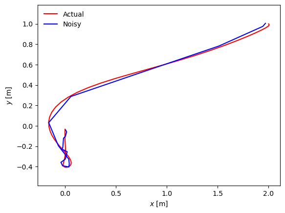
# Run a simulation with full state feedback (no noise) to generate a trajectory
uvec = [xd, ud, V, W*0]
lqr_resp = ct.input_output_response(lqr_clsys, timepts, uvec, x0)
U = lqr_resp.outputs[6:8] # controller input signals
Y = lqr_resp.outputs[0:3] + W # noisy output signals (noise in pvtol_noisy)
# Compare to the no noise case
uvec = [xd, ud, V*0, W*0]
lqr0_resp = ct.input_output_response(lqr_clsys, timepts, uvec, x0)
lqr0_fine = ct.input_output_response(lqr_clsys, timepts, uvec, x0,
t_eval=np.linspace(timepts[0], timepts[-1], 100))
U0 = lqr0_resp.outputs[6:8]
Y0 = lqr0_resp.outputs[0:3]
# Compare the results
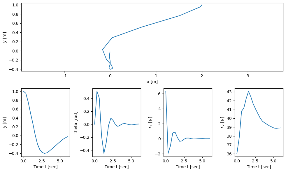
# plt.plot(Y0[0], Y0[1], 'k--', linewidth=2, label="No disturbances")
plt.plot(lqr0_fine.states[0], lqr0_fine.states[1], 'r-', label="Actual")
plt.plot(Y[0], Y[1], 'b-', label="Noisy")
plt.xlabel('$x$ [m]')
plt.ylabel('$y$ [m]')
plt.axis('equal')
plt.legend(frameon=False)
plt.figure()
plot_results(timepts, lqr_resp.states, lqr_resp.outputs[6:8]);
<Figure size 640x480 with 0 Axes>
[7]:
# Utility functions for making plots
def plot_state_comparison(
timepts, est_states, act_states=None, estimated_label='$\\hat x_{i}$', actual_label='$x_{i}$',
start=0):
for i in range(sys.nstates):
plt.subplot(2, 3, i+1)
if act_states is not None:
plt.plot(timepts[start:], act_states[i, start:], 'r--',
label=actual_label.format(i=i))
plt.plot(timepts[start:], est_states[i, start:], 'b',
label=estimated_label.format(i=i))
plt.legend()
plt.tight_layout()
# Define a function to plot out all of the relevant signals
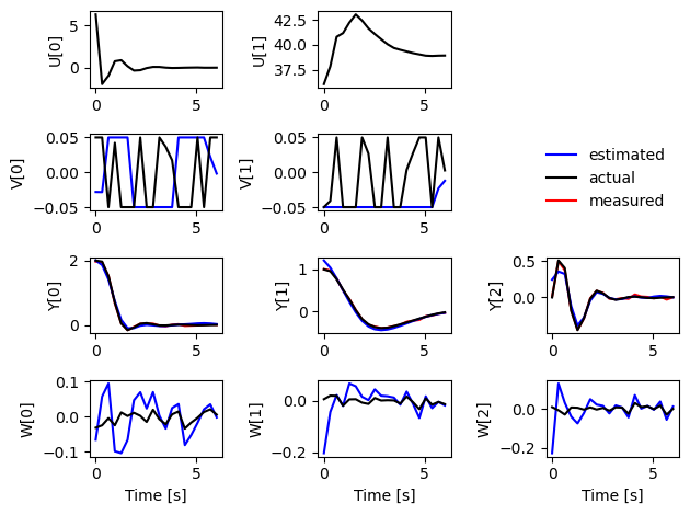
def plot_estimator_response(timepts, estimated, U, V, Y, W, start=0):
# Plot the input signal and disturbance
for i in [0, 1]:
# Input signal (the same across all)
plt.subplot(4, 3, i+1)
plt.plot(timepts[start:], U[i, start:], 'k')
plt.ylabel(f'U[{i}]')
# Plot the estimated disturbance signal
plt.subplot(4, 3, 4+i)
plt.plot(timepts[start:], estimated.inputs[i, start:], 'b-', label="est")
plt.plot(timepts[start:], V[i, start:], 'k', label="actual")
plt.ylabel(f'V[{i}]')
plt.subplot(4, 3, 6)
plt.plot(0, 0, 'b', label="estimated")
plt.plot(0, 0, 'k', label="actual")
plt.plot(0, 0, 'r', label="measured")
plt.legend(frameon=False)
plt.grid(False)
plt.axis('off')
# Plot the output (measured and estimated)
for i in [0, 1, 2]:
plt.subplot(4, 3, 7+i)
plt.plot(timepts[start:], Y[i, start:], 'r', label="measured")
plt.plot(timepts[start:], estimated.states[i, start:], 'b', label="measured")
plt.plot(timepts[start:], Y[i, start:] - W[i, start:], 'k', label="actual")
plt.ylabel(f'Y[{i}]')
for i in [0, 1, 2]:
plt.subplot(4, 3, 10+i)
plt.plot(timepts[start:], estimated.outputs[i, start:], 'b', label="estimated")
plt.plot(timepts[start:], W[i, start:], 'k', label="actual")
plt.ylabel(f'W[{i}]')
plt.xlabel('Time [s]')
plt.tight_layout()
State Estimation
[8]:
# Create a new system with only x, y, theta as outputs
# TODO: add this to pvtol.py?
sys = ct.NonlinearIOSystem(
    pvt._noisy_update, lambda t, x, u, params: x[0:3], name="pvtol_noisy",
    states = [f'x{i}' for i in range(6)],
    inputs = ['F1', 'F2'] + ['Dx', 'Dy'],
    outputs = ['x', 'y', 'theta']
)
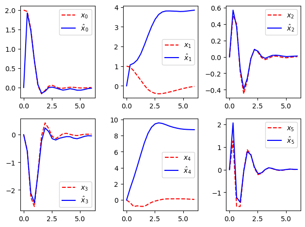
[9]:
# Standard Kalman filter
linsys = sys.linearize(xe, [ue, V[:, 0] * 0])
# print(linsys)
B = linsys.B[:, 0:2]
G = linsys.B[:, 2:4]
linsys = ct.ss(
    linsys.A, B, linsys.C, 0,
    states=sys.state_labels, inputs=sys.input_labels[0:2], outputs=sys.output_labels)
# print(linsys)

estim = ct.create_estimator_iosystem(linsys, Qv, Qw, G=G, P0=P0)
print(estim)
print(f'{xe=}, {P0=}')

kf_resp = ct.input_output_response(
    estim, timepts, [Y, U], X0 = [xe, P0.reshape(-1)])
plot_state_comparison(timepts, kf_resp.outputs, lqr_resp.states)
<NonlinearIOSystem>: sys[7]
Inputs (5): ['y[0]', 'y[1]', 'y[2]', 'F1', 'F2']
Outputs (6): ['xhat[0]', 'xhat[1]', 'xhat[2]', 'xhat[3]', 'xhat[4]', 'xhat[5]']
States (42): ['xhat[0]', 'xhat[1]', 'xhat[2]', 'xhat[3]', 'xhat[4]', 'xhat[5]', 'P[0,0]', 'P[0,1]', 'P[0,2]', 'P[0,3]', 'P[0,4]', 'P[0,5]', 'P[1,0]', 'P[1,1]', 'P[1,2]', 'P[1,3]', 'P[1,4]', 'P[1,5]', 'P[2,0]', 'P[2,1]', 'P[2,2]', 'P[2,3]', 'P[2,4]', 'P[2,5]', 'P[3,0]', 'P[3,1]', 'P[3,2]', 'P[3,3]', 'P[3,4]', 'P[3,5]', 'P[4,0]', 'P[4,1]', 'P[4,2]', 'P[4,3]', 'P[4,4]', 'P[4,5]', 'P[5,0]', 'P[5,1]', 'P[5,2]', 'P[5,3]', 'P[5,4]', 'P[5,5]']

Update: <function create_estimator_iosystem.<locals>._estim_update at 0x1685997e0>
Output: <function create_estimator_iosystem.<locals>._estim_output at 0x16859a4d0>
xe=array([ 0.000000e+00,  0.000000e+00,  0.000000e+00,  0.000000e+00,
       -1.766654e-27,  0.000000e+00]), P0=array([[1., 0., 0., 0., 0., 0.],
       [0., 1., 0., 0., 0., 0.],
       [0., 0., 1., 0., 0., 0.],
       [0., 0., 0., 1., 0., 0.],
       [0., 0., 0., 0., 1., 0.],
       [0., 0., 0., 0., 0., 1.]])
Extended Kalman filter
[10]:
# Define the disturbance input and measured output matrices
F = np.array([[0, 0], [0, 0], [0, 0], [1/pvtol.params['m'], 0], [0, 1/pvtol.params['m']], [0, 0]])
C = np.eye(3, 6)

Qwinv = np.linalg.inv(Qw)

# Estimator update law
def estimator_update(t, x, u, params):
    # Extract the states of the estimator
    xhat = x[0:pvtol.nstates]
    P = x[pvtol.nstates:].reshape(pvtol.nstates, pvtol.nstates)

    # Extract the inputs to the estimator
    y = u[0:3]                  # just grab the first three outputs
    u = u[6:8]                  # get the inputs that were applied as well

    # Compute the linearization at the current state
    A = pvtol.A(xhat, u)        # A matrix depends on current state
    # A = pvtol.A(xe, ue)       # Fixed A matrix (for testing/comparison)

    # Compute the optimal "gain
    L = P @ C.T @ Qwinv

    # Update the state estimate
    xhatdot = pvtol.updfcn(t, xhat, u, params) - L @ (C @ xhat - y)

    # Update the covariance
    Pdot = A @ P + P @ A.T - P @ C.T @ Qwinv @ C @ P + F @ Qv @ F.T

    # Return the derivative
    return np.hstack([xhatdot, Pdot.reshape(-1)])

def estimator_output(t, x, u, params):
    # Return the estimator states
    return x[0:pvtol.nstates]

ekf = ct.NonlinearIOSystem(
    estimator_update, estimator_output,
    states=pvtol.nstates + pvtol.nstates**2,
    inputs= pvtol_noisy.output_labels \
        + pvtol_noisy.input_labels[0:pvtol.ninputs],
    outputs=[f'xh{i}' for i in range(pvtol.nstates)]
)
print(ekf)
<NonlinearIOSystem>: sys[8]
Inputs (8): ['x0', 'x1', 'x2', 'x3', 'x4', 'x5', 'F1', 'F2']
Outputs (6): ['xh0', 'xh1', 'xh2', 'xh3', 'xh4', 'xh5']
States (42): ['x[0]', 'x[1]', 'x[2]', 'x[3]', 'x[4]', 'x[5]', 'x[6]', 'x[7]', 'x[8]', 'x[9]', 'x[10]', 'x[11]', 'x[12]', 'x[13]', 'x[14]', 'x[15]', 'x[16]', 'x[17]', 'x[18]', 'x[19]', 'x[20]', 'x[21]', 'x[22]', 'x[23]', 'x[24]', 'x[25]', 'x[26]', 'x[27]', 'x[28]', 'x[29]', 'x[30]', 'x[31]', 'x[32]', 'x[33]', 'x[34]', 'x[35]', 'x[36]', 'x[37]', 'x[38]', 'x[39]', 'x[40]', 'x[41]']

Update: <function estimator_update at 0x1685100d0>
Output: <function estimator_output at 0x168512170>
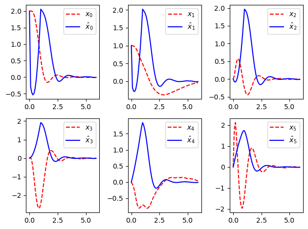
[11]:
ekf_resp = ct.input_output_response(
    ekf, timepts, [lqr_resp.states, lqr_resp.outputs[6:8]],
    X0=[xe, P0.reshape(-1)])
plot_state_comparison(timepts, ekf_resp.outputs, lqr_resp.states)
[12]:
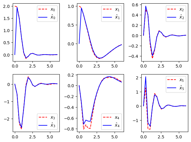
# Define the optimal estimation problem
traj_cost = opt.gaussian_likelihood_cost(sys, Qv, Qw)
init_cost = lambda xhat, x: (xhat - x) @ P0 @ (xhat - x)
oep = opt.OptimalEstimationProblem(
sys, timepts, traj_cost, terminal_cost=init_cost)
# Compute the estimate from the noisy signals
est = oep.compute_estimate(Y, U, X0=lqr_resp.states[:, 0])
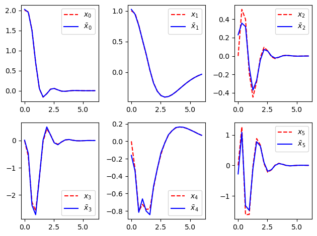
plot_state_comparison(timepts, est.states, lqr_resp.states)
Summary statistics:
* Cost function calls: 5051
* Final cost: 354.3319137685172
[13]:
# Plot the response of the estimator
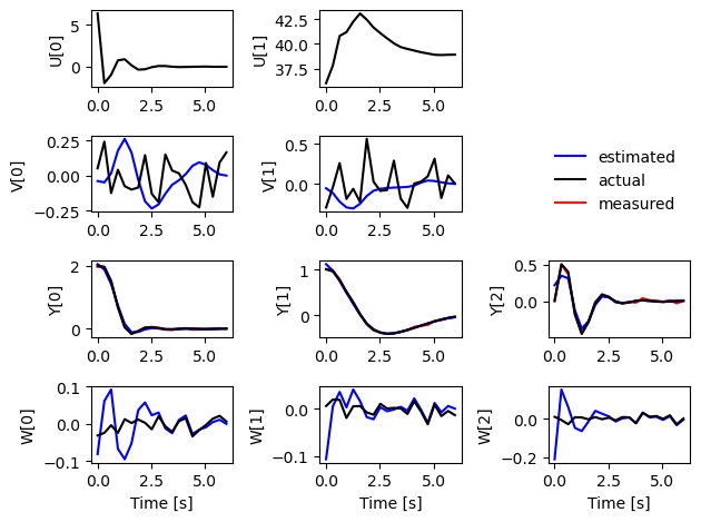
plot_estimator_response(timepts, est, U, V, Y, W)
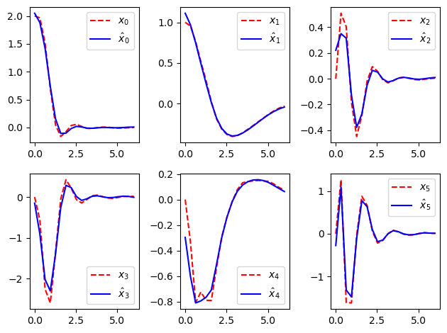
[14]:
# Noise free and disturbance free => estimation should be near perfect
noisefree_cost = opt.gaussian_likelihood_cost(sys, Qv, Qw*1e-6)
oep0 = opt.OptimalEstimationProblem(
        sys, timepts, noisefree_cost, terminal_cost=init_cost)
est0 = oep0.compute_estimate(Y0, U0, X0=lqr0_resp.states[:, 0],
                            initial_guess=(lqr0_resp.states, V * 0))
plot_state_comparison(
    timepts, est0.states, lqr0_resp.states, estimated_label='$\\bar x_{i}$')
Summary statistics:
* Cost function calls: 9464
* Final cost: 212754409.97292745
[15]:
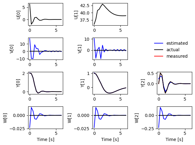
plot_estimator_response(timepts, est0, U0, V*0, Y0, W*0)
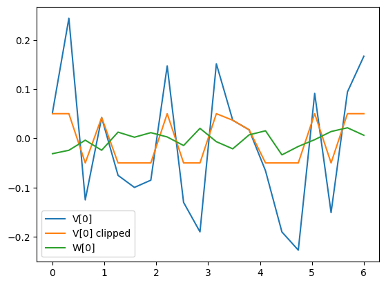
Bounded disturbances
Another thing that the MHE can handled is input distributions that are bounded. We implement that here by carrying out the optimal estimation problem with constraints.
[16]:
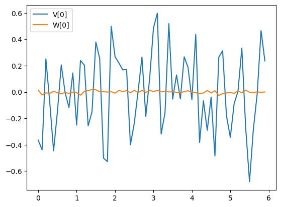
V_clipped = np.clip(V, -0.05, 0.05)

plt.plot(timepts, V[0], label="V[0]")
plt.plot(timepts, V_clipped[0], label="V[0] clipped")
plt.plot(timepts, W[0], label="W[0]")
plt.legend();
[17]:
uvec = [xe, ue, V_clipped, W]
clipped_resp = ct.input_output_response(lqr_clsys, timepts, uvec, x0)
U_clipped = clipped_resp.outputs[6:8] # controller input signals
Y_clipped = clipped_resp.outputs[0:3] + W # noisy output signals
traj_constraint = opt.disturbance_range_constraint(
sys, [-0.05, -0.05], [0.05, 0.05])
oep_clipped = opt.OptimalEstimationProblem(
sys, timepts, traj_cost, terminal_cost=init_cost,
trajectory_constraints=traj_constraint)
est_clipped = oep_clipped.compute_estimate(
Y_clipped, U_clipped, X0=lqr0_resp.states[:, 0])
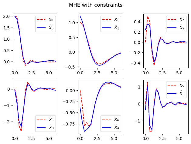
plot_state_comparison(timepts, est_clipped.states, lqr_resp.states)
plt.suptitle("MHE with constraints")
plt.tight_layout()
plt.figure()
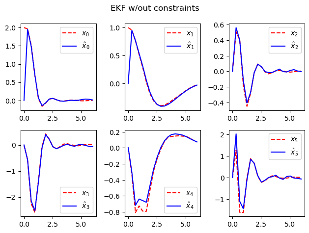
ekf_unclipped = ct.input_output_response(
ekf, timepts, [clipped_resp.states, clipped_resp.outputs[6:8]],
X0=[xe, P0.reshape(-1)])
plot_state_comparison(timepts, ekf_unclipped.outputs, lqr_resp.states)
plt.suptitle("EKF w/out constraints")
plt.tight_layout()
Summary statistics:
* Cost function calls: 3572
* Constraint calls: 3756
* Final cost: 531.7451775567271
[18]:
plot_estimator_response(timepts, est_clipped, U, V_clipped, Y, W)
Moving Horizon Estimation (MHE)
We can now move to implementation of a moving horizon estimator, using our fixed horizon optimal estimator.
[19]:
# Use a shorter horizon
mhe_timepts = timepts[0:5]
oep = opt.OptimalEstimationProblem(
        sys, mhe_timepts, traj_cost, terminal_cost=init_cost)

try:
    mhe = oep.create_mhe_iosystem(2)

    est_mhe = ct.input_output_response(
        mhe, timepts, [Y, U], X0=resp.states[:, 0],
        params={'verbose': True}
    )
    plot_state_comparison(timepts, est_mhe.states, lqr_resp.states)
except:
    print("MHE for continuous time systems not implemented")
MHE for continuous time systems not implemented
[20]:
# Create discrete time version of PVTOL
Ts = 0.1
print(f"Sample time: {Ts=}")
dsys = ct.NonlinearIOSystem(
    lambda t, x, u, params: x + Ts * sys.updfcn(t, x, u, params),
    sys.outfcn, dt=Ts, states=sys.state_labels,
    inputs=sys.input_labels, outputs=sys.output_labels,
)
print(dsys)
Sample time: Ts=0.1
<NonlinearIOSystem>: sys[9]
Inputs (4): ['F1', 'F2', 'Dx', 'Dy']
Outputs (3): ['x', 'y', 'theta']
States (6): ['x0', 'x1', 'x2', 'x3', 'x4', 'x5']

Update: <function <lambda> at 0x168af1360>
Output: <function <lambda> at 0x168598940>
[21]:
# Create a new list of time points
timepts = np.arange(0, Tf, Ts)

# Create representative process disturbance and sensor noise vectors
# np.random.seed(117)           # avoid figures changing from run to run
V = ct.white_noise(timepts, Qv)
# V = np.clip(V0, -0.1, 0.1)    # Hold for later
W = ct.white_noise(timepts, Qw, dt=Ts)
# plt.plot(timepts, V0[0], 'b--', label="V[0]")
plt.plot(timepts, V[0], label="V[0]")
plt.plot(timepts, W[0], label="W[0]")
plt.legend();
[22]:
# Generate a new trajectory over the longer time vector
uvec = [xd, ud, V, W*0]
lqr_resp = ct.input_output_response(lqr_clsys, timepts, uvec, x0)
U = lqr_resp.outputs[6:8]                    # controller input signals
Y = lqr_resp.outputs[0:3] + W                # noisy output signals
[23]:
mhe_timepts = timepts[0:10]
oep = opt.OptimalEstimationProblem(
        dsys, mhe_timepts, traj_cost, terminal_cost=init_cost,
        disturbance_indices=slice(2, 4))
mhe = oep.create_mhe_iosystem()

mhe_resp = ct.input_output_response(
    mhe, timepts, [Y, U], X0=x0,
    params={'verbose': True}
)
plot_state_comparison(timepts, mhe_resp.states, lqr_resp.states)
[24]:
# Resimulate starting at the origin and moving to the "initial" condition
uvec = [x0, ue, V, W*0]
lqr_resp = ct.input_output_response(lqr_clsys, timepts, uvec, xe)
U = lqr_resp.outputs[6:8]                    # controller input signals
Y = lqr_resp.outputs[0:3] + W                # noisy output signals
[25]:
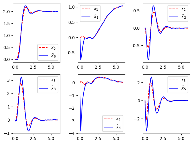
mhe_timepts = timepts[0:8]
oep = opt.OptimalEstimationProblem(
        dsys, mhe_timepts, traj_cost, terminal_cost=init_cost,
        disturbance_indices=slice(2, 4))
mhe = oep.create_mhe_iosystem()

mhe_resp = ct.input_output_response(
    mhe, timepts, [Y, U],
    params={'verbose': True}
)
plot_state_comparison(timepts, mhe_resp.outputs, lqr_resp.states)
[ ]: