Interconnect Tutorial
Sawyer B. Fuller 2023.04
Goal: Create a single dynamic system that implements a complicated interconnected (ie, realistic) system such as the following:
-system-such-as-the-following:image.png)
[1]:
import numpy as np # numerical library
import matplotlib.pyplot as plt # plotting library
import control as ct # control systems library
preliminaries
The representation of all systems in the interconnected system will be a linear, time-invariant system in state-space form given by
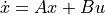 ,
, 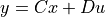
for continuous-time systems, and
![x[k+1] = Ax[k]+Bu[k]](_images/math/8ef626c1360a755725adf7e10073ca4cb2a4abee.png)
![~~~~~~~y[k]=Cx[k]+Du[k]](_images/math/b57a8208c8d1bea9b511a895878bebe68c992080.png)
for discrete-time systems.  is the state,
  is the input, and
  is the output. All of which are possibly vector-valued.
auto-splitting
A signal is automatically routed into every system that has an input of the same name
     u        y1
u  +--> sys1 --->
---|
   +--> sys2 --->
     u        y2
[2]:
# arbitrary example systems
sys1 = ct.tf(1, [10, 1], inputs='u', outputs='y1')
sys2 = ct.tf(1, [1, 0], inputs='u', outputs='y2')

# create interconnected system
interconnected = ct.interconnect([sys1, sys2], inputs='u', outputs=['y1', 'y2'])
display(interconnected) # 1-input, 2-output system
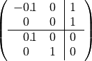
For this system, the input has a single value ![[u]](_images/math/8bcf8acf8fbf9092c408a076f0e6e31c841e0c48.png) , while the output is a two-element vector
, while the output is a two-element vector ![y=[y1, y2]^T](_images/math/87e95d39ba922c8ea28b37326d0325435bb9d1bc.png) .
.
auto-summing
Systems with output signals of the same name are automatically added.
  u1        y
---> sys1 ---+
             |
           + V    y
             O----->
           + ^
             |
---> sys2 ---+
  u1        y
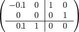
[3]:
sys1 = ct.tf(1, [10, 1], inputs='u1', outputs='y')
sys2 = ct.tf(1, [1, 0], inputs='u2', outputs='y')

# create interconnected system
interconnected = ct.interconnect([sys1, sys2], inplist=['u1', 'u2'], outlist='y')
display(interconnected) #  2-input, 1-output system
summing junctions
Use a summing junction to interconnect signals of different names, or to change the sign of a signal.
 u      w
---> O --->
     ^
     | -v
     |
[4]:
summer = ct.summing_junction(['u', '-v'], 'w') # w = u - v
display(summer)

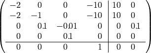
constructing the goal system depicted above
[5]:
# constants
K = 10
zc = 0.001 # controller zero location
pc = 2 # controller pole location
tau = 1
J = 100
b = 1

# systems
C = ct.tf([K, K*zc],[1, pc], inputs='e', outputs='u')
lopass = ct.tf(1, [tau, 1], inputs='u', outputs='v')
P = ct.tf(1, [J, b], inputs='w', outputs='thetadot')
integrator = ct.tf(1, [1, 0], inputs='thetadot', outputs='theta')
error = ct.summing_junction(['thetaref', '-theta'], 'e') # e = thetaref-theta
disturbance = ct.summing_junction(['d', 'v'], 'w') # w = d+v

# interconnect everything based on signal names
sys = ct.interconnect([C, lopass, P, integrator, error, disturbance],
                       inputs=['thetaref', 'd'], outputs='theta')
display(sys)
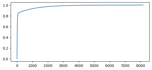
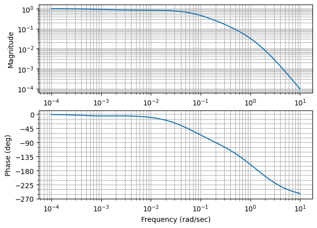
Finally, we can use the interconnected system just like we would use any other system object, such as computing step and frequency responses.
[6]:
# extract system input-output pairs
# index order is [output, input]
plt.figure(figsize=(7,3))
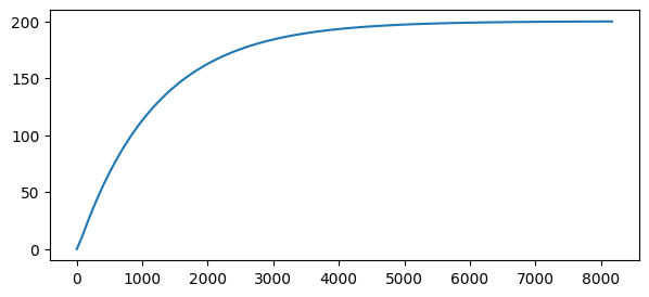
sys_thetaref_to_theta = sys[0, 0]
sys_d_to_theta = sys[0, 1]
t, y = ct.step_response(sys_thetaref_to_theta) # step response
plt.plot(t,y)
plt.figure(figsize=(7,3))
t, yd = ct.step_response(sys_d_to_theta) # disturbance response
plt.plot(t,yd);
plt.figure(figsize=(7,5))
ct.bode_plot(sys_thetaref_to_theta, plot=True);