Input/output systems
Module usage
An input/output system is defined as a dynamical system that has a system
state as well as inputs and outputs (either inputs or states can be empty).
The dynamics of the system can be in continuous or discrete time. To simulate
an input/output system, use the input_output_response()
function:
t, y = ct.input_output_response(io_sys, T, U, X0, params)
An input/output system can be linearized around an equilibrium point to obtain
a StateSpace linear system. Use the
find_eqpt() function to obtain an equilibrium point and the
linearize() function to linearize about that equilibrium point:
xeq, ueq = ct.find_eqpt(io_sys, X0, U0)
ss_sys = ct.linearize(io_sys, xeq, ueq)
Input/output systems are automatically created for state space LTI systems
when using the ss() function. Nonlinear input/output systems can be
created using the NonlinearIOSystem class, which requires
the definition of an update function (for the right hand side of the
differential or different equation) and an output function (computes the
outputs from the state):
io_sys = NonlinearIOSystem(updfcn, outfcn, inputs=M, outputs=P, states=N)
More complex input/output systems can be constructed by using the
interconnect() function, which allows a collection of
input/output subsystems to be combined with internal connections
between the subsystems and a set of overall system inputs and outputs
that link to the subsystems:
steering = ct.interconnect(
    [plant, controller], name='system',
    connections=[['controller.e', '-plant.y']],
    inplist=['controller.e'], inputs='r',
    outlist=['plant.y'], outputs='y')
Interconnected systems can also be created using block diagram manipulations
such as the series(), parallel(), and
feedback() functions. The InputOutputSystem
class also supports various algebraic operations such as * (series
interconnection) and + (parallel interconnection).
Example
To illustrate the use of the input/output systems module, we create a model for a predator/prey system, following the notation and parameter values in FBS2e.
We begin by defining the dynamics of the system
import control as ct
import numpy as np
import matplotlib.pyplot as plt

def predprey_rhs(t, x, u, params):
    # Parameter setup
    a = params.get('a', 3.2)
    b = params.get('b', 0.6)
    c = params.get('c', 50.)
    d = params.get('d', 0.56)
    k = params.get('k', 125)
    r = params.get('r', 1.6)

    # Map the states into local variable names
    H = x[0]
    L = x[1]

    # Compute the control action (only allow addition of food)
    u_0 = u[0] if u[0] > 0 else 0

    # Compute the discrete updates
    dH = (r + u_0) * H * (1 - H/k) - (a * H * L)/(c + H)
    dL = b * (a * H *  L)/(c + H) - d * L

    return np.array([dH, dL])
We now create an input/output system using these dynamics:
io_predprey = ct.NonlinearIOSystem(
    predprey_rhs, None, inputs=('u'), outputs=('H', 'L'),
    states=('H', 'L'), name='predprey')
Note that since we have not specified an output function, the entire state will be used as the output of the system.
The io_predprey system can now be simulated to obtain the open loop dynamics of the system:
X0 = [25, 20]                 # Initial H, L
T = np.linspace(0, 70, 500)   # Simulation 70 years of time

# Simulate the system
t, y = ct.input_output_response(io_predprey, T, 0, X0)

# Plot the response
plt.figure(1)
plt.plot(t, y[0])
plt.plot(t, y[1])
plt.legend(['Hare', 'Lynx'])
plt.show(block=False)
We can also create a feedback controller to stabilize a desired population of the system. We begin by finding the (unstable) equilibrium point for the system and computing the linearization about that point.
eqpt = ct.find_eqpt(io_predprey, X0, 0)
xeq = eqpt[0]                         # choose the nonzero equilibrium point
lin_predprey = ct.linearize(io_predprey, xeq, 0)
We next compute a controller that stabilizes the equilibrium point using eigenvalue placement and computing the feedforward gain using the number of lynxes as the desired output (following FBS2e, Example 7.5):
K = ct.place(lin_predprey.A, lin_predprey.B, [-0.1, -0.2])
A, B = lin_predprey.A, lin_predprey.B
C = np.array([[0, 1]])                # regulated output = number of lynxes
kf = -1/(C @ np.linalg.inv(A - B @ K) @ B)
To construct the control law, we build a simple input/output system that applies a corrective input based on deviations from the equilibrium point. This system has no dynamics, since it is a static (affine) map, and can constructed using the ~control.ios.NonlinearIOSystem class:
io_controller = ct.NonlinearIOSystem(
  None,
  lambda t, x, u, params: -K @ (u[1:] - xeq) + kf * (u[0] - xeq[1]),
  inputs=('Ld', 'u1', 'u2'), outputs=1, name='control')
The input to the controller is u, consisting of the vector of hare and lynx populations followed by the desired lynx population.
To connect the controller to the predatory-prey model, we create an
InterconnectedSystem using the interconnect()
function:
io_closed = ct.interconnect(
  [io_predprey, io_controller],       # systems
  connections=[
    ['predprey.u', 'control.y[0]'],
    ['control.u1',  'predprey.H'],
    ['control.u2',  'predprey.L']
  ],
  inplist=['control.Ld'],
  outlist=['predprey.H', 'predprey.L', 'control.y[0]']
)
Finally, we simulate the closed loop system:
# Simulate the system
t, y = ct.input_output_response(io_closed, T, 30, [15, 20])

# Plot the response
plt.figure(2)
plt.subplot(2, 1, 1)
plt.plot(t, y[0])
plt.plot(t, y[1])
plt.legend(['Hare', 'Lynx'])
plt.subplot(2, 1, 2)
plt.plot(t, y[2])
plt.legend(['input'])
plt.show(block=False)
Additional features
The I/O systems module has a number of other features that can be used to simplify the creation of interconnected input/output systems.
Summing junction
The summing_junction() function can be used to create an
input/output system that takes the sum of an arbitrary number of inputs. For
example, to create an input/output system that takes the sum of three inputs,
use the command
sumblk = ct.summing_junction(3)
By default, the name of the inputs will be of the form u[i] and the output
will be y. This can be changed by giving an explicit list of names:
sumblk = ct.summing_junction(inputs=['a', 'b', 'c'], output='d')
A more typical usage would be to define an input/output system that compares a reference signal to the output of the process and computes the error:
sumblk = ct.summing_junction(inputs=['r', '-y'], output='e')
Note the use of the minus sign as a means of setting the sign of the input ‘y’ to be negative instead of positive.
It is also possible to define “vector” summing blocks that take multi-dimensional inputs and produce a multi-dimensional output. For example, the command
sumblk = ct.summing_junction(inputs=['r', '-y'], output='e', dimension=2)
will produce an input/output block that implements e[0] = r[0] - y[0] and
e[1] = r[1] - y[1].
Automatic connections using signal names
The interconnect() function allows the interconnection of
multiple systems by using signal names of the form sys.signal. In many
situations, it can be cumbersome to explicitly connect all of the appropriate
inputs and outputs. As an alternative, if the connections keyword is
omitted, the interconnect() function will connect all signals
of the same name to each other. This can allow for simplified methods of
interconnecting systems, especially when combined with the
summing_junction() function. For example, the following code
will create a unity gain, negative feedback system:
P = ct.tf2io([1], [1, 0], inputs='u', outputs='y')
C = ct.tf2io([10], [1, 1], inputs='e', outputs='u')
sumblk = ct.summing_junction(inputs=['r', '-y'], output='e')
T = ct.interconnect([P, C, sumblk], inplist='r', outlist='y')
If a signal name appears in multiple outputs then that signal will be summed
when it is interconnected. Similarly, if a signal name appears in multiple
inputs then all systems using that signal name will receive the same input.
The interconnect() function will generate an error if an signal
listed in inplist or outlist (corresponding to the inputs and outputs
of the interconnected system) is not found, but inputs and outputs of
individual systems that are not connected to other systems are left
unconnected (so be careful!).
Automated creation of state feedback systems
The create_statefbk_iosystem() function can be used to
create an I/O system consisting of a state feedback gain (with
optional integral action and gain scheduling) and an estimator. A
basic state feedback controller of the form
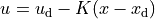
can be created with the command:
ctrl, clsys = ct.create_statefbk_iosystem(sys, K)
where sys is the process dynamics and K is the state feedback gain
(e.g., from LQR). The function returns the controller ctrl and the
closed loop systems clsys, both as I/O systems. The input to the
controller is the vector of desired states  , desired
inputs
, desired
inputs  , and system states
  .
.
If the full system state is not available, the output of a state estimator can be used to construct the controller using the command:
ctrl, clsys = ct.create_statefbk_iosystem(sys, K, estimator=estim)
where estim is the state estimator I/O system. The controller will
have the same form as above, but with the system state
replaced by the estimated state  (output of estim).
The closed loop controller will include both the state feedback and
the estimator.
(output of estim).
The closed loop controller will include both the state feedback and
the estimator.
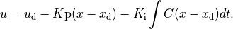
Integral action can be included using the integral_action keyword.
The value of this keyword can either be an matrix (ndarray) or a
function. If a matrix  is specified, the difference between
the desired state and system state will be multiplied by this matrix
and integrated. The controller gain should then consist of a set of
proportional gains
is specified, the difference between
the desired state and system state will be multiplied by this matrix
and integrated. The controller gain should then consist of a set of
proportional gains  and integral gains
 with
with

and the control action will be given by
If integral_action is a function h, that function will be called
with the signature h(t, x, u, params) to obtain the outputs that
should be integrated. The number of outputs that are to be integrated
must match the number of additional columns in the K matrix. If an
estimator is specified, will be used in place of
.
Finally, gain scheduling on the desired state, desired input, or system state can be implemented by setting the gain to a 2-tuple consisting of a list of gains and a list of points at which the gains were computed, as well as a description of the scheduling variables:
ctrl, clsys = ct.create_statefbk_iosystem(
    sys, ([g1, ..., gN], [p1, ..., pN]), gainsched_indices=[s1, ..., sq])
The list of indices can either be integers indicating the offset into
the controller input vector  or a
list of strings matching the names of the input signals. The
controller implemented in this case has the form
or a
list of strings matching the names of the input signals. The
controller implemented in this case has the form
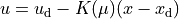
where  represents the scheduling variables. See
Gain scheduled control for vehicle steeering (I/O system) for an example implementation of a gain
scheduled controller (in the alternative formulation section at the
bottom of the file).
represents the scheduling variables. See
Gain scheduled control for vehicle steeering (I/O system) for an example implementation of a gain
scheduled controller (in the alternative formulation section at the
bottom of the file).
Integral action and state estimation can also be used with gain scheduled controllers.
Module classes and functions
|
A class for representing input/output systems. |
|
Interconnection of a set of input/output systems. |
|
Interconnection of a set of linear input/output systems. |
|
Input/output representation of a linear (state space) system. |
|
Nonlinear I/O system. |
|
Find the equilibrium point for an input/output system. |
|
Linearize an input/output system at a given state and input. |
|
Compute the output response of a system to a given input. |
|
Interconnect a set of input/output systems. |
|
Create an I/O system from a state space linear system. |
|
Create a summing junction as an input/output system. |
|
Convert a transfer function into an I/O system |